7.4. Performance Optimization Methods
Hardware accelerators boast intricate computational and memory architectures. To maximize their performance, developers frequently need to grasp a variety of performance optimization methods. Common methods encompass enhancing arithmetic intensity, capitalizing effectively on shared memory, optimizing the memory load/store pipeline, among others. The subsequent sections will elucidate these methods through practical programming examples, all aimed towards a singular objective: accelerating an FP32 GEMM program.
7.4.1. Implementing General Matrix Multiplication
Code lst:cpu shows a reference implementation of GEMM in C++.
lst:cpu
float A[M][K];
float B[K][N];
float C[M][N];
float alpha, beta;

for (unsigned m = 0; m < M; ++m) {
    for (unsigned n = 0; n < N; ++n) {
        float c = 0;
        for (unsigned k = 0; k < K; ++k) {
            c += A[m][k] * B[k][n];
        }
        C[m][n] = alpha * c + beta * C[m][n];
    }
}
ach element in matrix \(C\) is independently computed, and numerous
GPU threads can be launched to compute the corresponding elements in
matrix \(C\) in parallel. The GPU kernel function is shown in
Code lst:gpu.
lst:gpu
__global__ void gemmKernel(const float * A,
const float * B, float * C,
float alpha, float beta, unsigned M, unsigned N,
unsigned K) {
    unsigned int m = threadIdx.x + blockDim.x * blockIdx.x;
    unsigned int n = threadIdx.y + blockDim.y * blockIdx.y;
    if (m >= M || n >= N)
    return;
    float c = 0;
    for (unsigned k = 0; k < K; ++k) {
        c += A[m * K + k] * B[k * N + n];
    }
    c = c * alpha;
    float result = c;
    if (beta != 0) {
        result = result + C[m * N + n] * beta;
    }
    C[m * N + n] = result;
}
Figure :numref:cuda_naive_gemm shows the layout of the
implementation. Each element in matrix \(C\) is computed by one
thread. The row index \(m\) and column index \(n\) of the
element in matrix \(C\) corresponding to the thread are computed in
lines 5 and 6 of the GPU kernel. Then, in lines 9 to 11, the thread
loads the row vector in matrix \(A\) according to the row index and
the column vector in matrix \(B\) according to the column index,
computes the vector inner product. The thread also stores the result
back to \(C\) matrix in line 17.
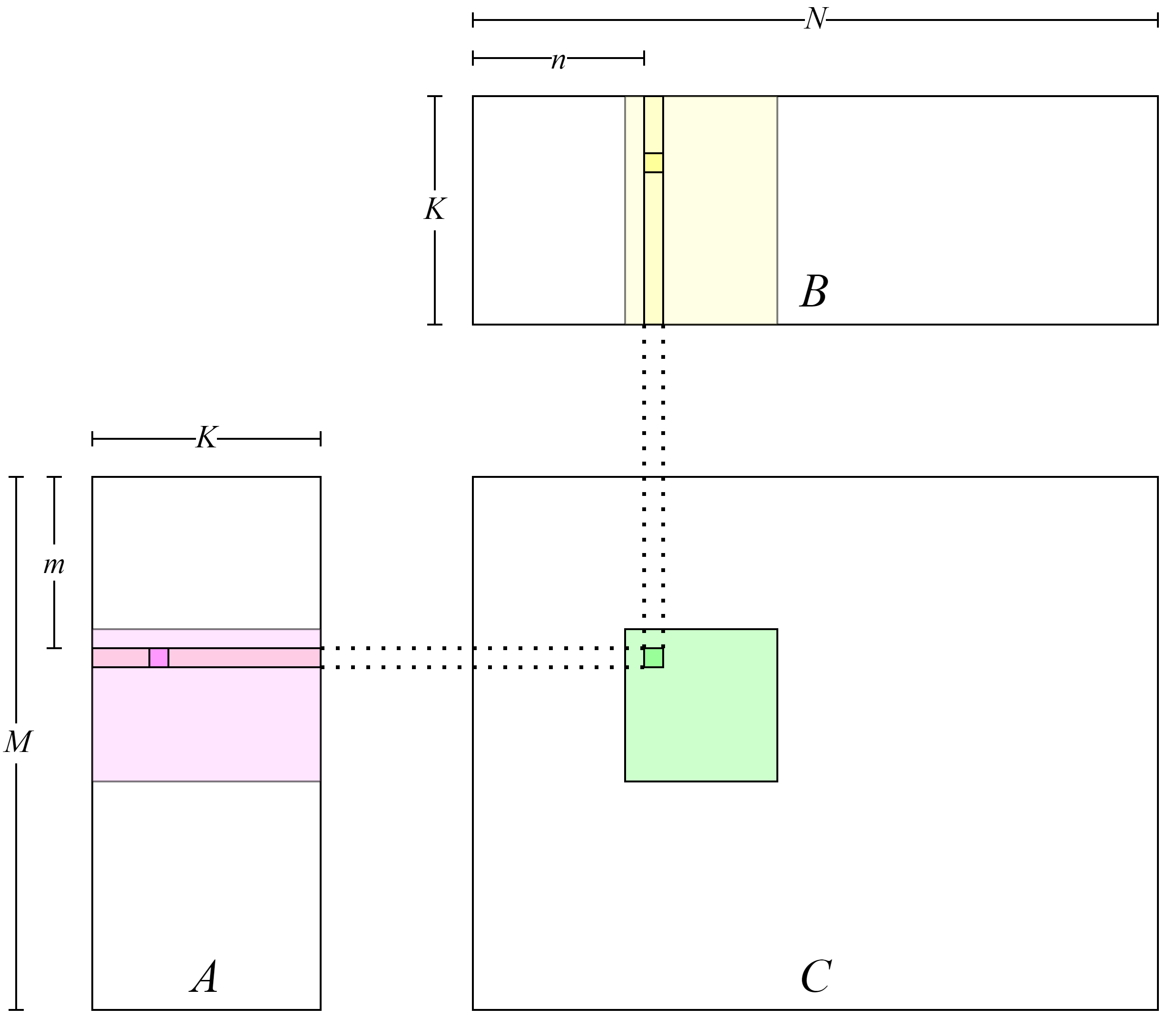
Fig. 7.4.1 Simple implementation ofGEMM
The method of launching the kernel function is shown in
Code lst:launch.
lst:launch
void gemmNaive(const float *A, const float *B, float *C,
float alpha, float beta, unsigned M,
unsigned N, unsigned K) {
    dim3 block(16, 16);
    dim3 grid((M - 1) / block.x + 1, (N - 1) / block.y + 1);

    gemmKernel<<<grid, block>>>(A, B, C, alpha, beta, M, N, K);
}
Each thread block processes \(16\times16\) elements in matrix \(C\). Therefore, \((M - 1) / 16 + 1 \times (N - 1) / 16 + 1\) thread blocks are used to compute the entire matrix \(C\).
Eigen is used to generate data and compute the GEMM result on the CPU. In addition, error computing and time profiling code are implemented for the GPU computing result. For details, see first_attempt.cu. After the program is compiled and executed, output results are as follows:
Average time: 48.961 ms
Max error: 0.000092
The peak GPU throughput can be approximated by using the following formula: 2 \(\times\) Frequency \(\times\) Number of single-precision compute units. The number of single-precision compute units equals the number of SMs in the GPU multiplied by the number of single-precision compute units in each SM. The results are as follows:
FP32 peak throughput 29767.680 GFLOPS
Average Throughput: 185.313 GFLOPS
A significant gap exists between the performance that can be achieved by the current code and the peak device performance. In an entire computing process, the process with the highest computing density is matrix multiplication \(A\times B\). Its time complexity is \(O(M*N*K)\), whereas that time complexity of the entire computing process is \(O(M*N*K+2*M*N)\). Therefore, optimizing matrix multiplication is key to improving performance.
7.4.2. Enhancing Arithmetic Intensity
Arithmetic intensity is the ratio of computational instructions to load/store instructions. Modern GPUs typically have numerous compute units, constrained only by a limited load/store bandwidth. This limitation often leaves these units waiting for data loading in a program. Thus, boosting arithmetic intensity is a crucial step to improve program performance.
In the GPU kernel function discussed previously, we can approximate its arithmetic intensity by dividing the total number of floating-point operations by the number of data reads. When calculating the inner product within \(K\) loops, floating-point multiplication and addition operations occur each time elements from matrix \(A\) and \(B\) are loaded. Consequently, the arithmetic intensity is 1, derived from two 32-bit floating-point operations divided by two 32-bit data load/store instructions.
In the original code, each thread handles one element in matrix \(C\), computing the inner product of a row in matrix \(A\) and a column in matrix \(B\). In essence, we can elevate the arithmetic intensity by amplifying the elements in matrix \(C\) that each thread can process, computing the inner product of multiple rows in matrix \(A\) and multiple columns in matrix \(B\). More specifically, if \(m\) elements in matrix \(A\) and \(n\) elements in matrix \(B\) are loaded concurrently while calculating the inner product in \(K\) loops, there are \(m+n\) 32-bit load/store instructions and \(2mn\) 32-bit computational instructions. Hence, the arithmetic intensity becomes \(\frac{2mn}{m+n}\). Therefore, by increasing \(m\) and \(n\), we can optimize the arithmetic intensity.
In the preceding section, a float pointer was employed to access
global memory and store data in it, utilizing the hardware instructions
LDG.E and STG.E. Multiple float elements can be loaded
concurrently using the 128-bit wide instructions LDG.E.128 and
STG.E.128. These wide instructions can streamline the instruction
sequence, potentially saving dozens of instruction issue cycles compared
to four standard instructions, thereby enabling the issue of more
computational instructions within the saved time. Wide instructions can
also enhance the cache line hit rate. Despite these benefits, we advise
against the blanket use of wide instructions in all code. Instead,
programmers should prioritize direct optimization methods, such as
parallel design and local data reuse.
A specific implementation is stacking four float numbers to form a
128-bit float4 class. The load/store operations will be completed
using a wide instruction for the float4 class. For details about the
code implementation, see
util.cuh.
Note that each thread needs to load four float numbers (instead of
one) from matrix \(A\) and matrix \(B\), requiring each thread
to process \(4\times 4\) blocks (thread tile) in matrix
\(C\). Each thread loads data from matrix \(A\) and matrix
\(B\) from left to right and from top to bottom, computes the data,
and stores the data to matrix \(C\), as shown in
Figure :numref:use_float4.
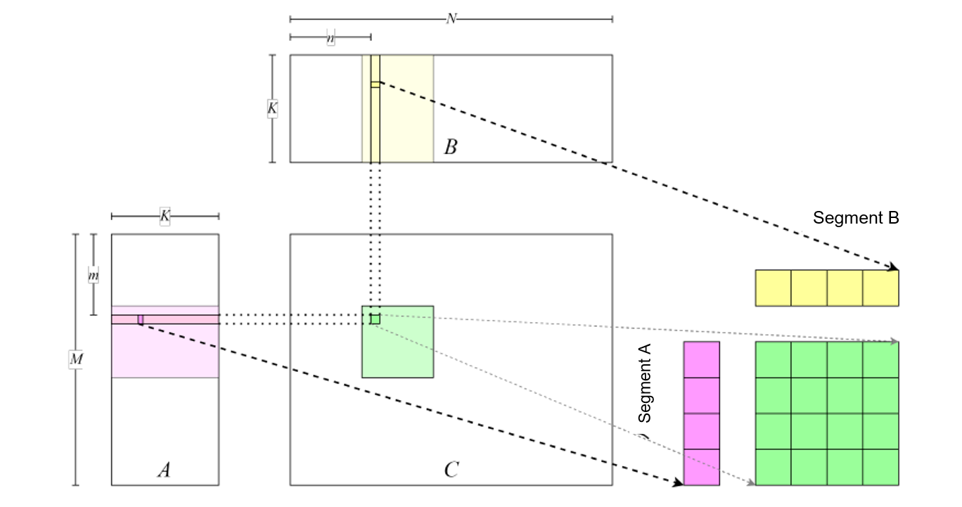
Fig. 7.4.2 Enhancing arithmeticintensity
For details about the complete code, see
gemm_use_128.cu.
We can further increase the amount of data processed by each thread in
order to improve the arithmetic intensity more, as shown in
Figure :numref:use_tile. For details about the code used to
achieve this, see
gemm_use_tile.cu.
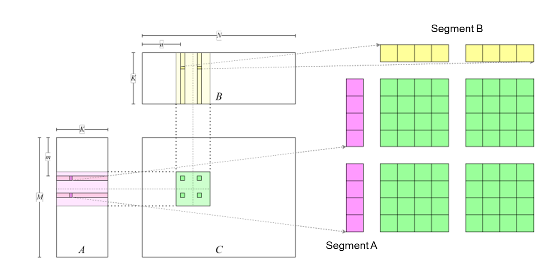
Fig. 7.4.3 Further enhancement of the arithmetic intensity by adding matrixblocks processed by eachthread
The test results are as follows:
Max Error: 0.000092
Average Time: 6.232 ms, Average Throughput: 1378.317 GFLOPS
To sample and analyze performance indicators, we will use the analysis tool Nsight Compute released by NVIDIA. This tool, designed for GPU kernel functions, samples and collects GPU activity data by hooking drivers. The following commands can be used to analyze the performance:
bash
ncu --set full -o <profile_output_file> <profile_process>
–set full indicates that all data is sampled. -o indicates that
the result is output as a file. <profile_output_file> indicates the
output file name without the file name extension. <profile_process>
indicates the executable file to be analyzed and its arguments. For
example, to analyze first_attempt and name the output result
first_attepmt_prof_result, run the following instructions:
ncu --set full -o first_attepmt_prof_result ./first_attempt
If the system displays a message indicating that you do not have
permission to run this command, prefix it with sudo and run it
again. After obtaining the output file, the program nv-nsight-cu can
be used to view the file. We compared the profiling results of the new
GPU kernel function and the previous one.
The result shows that the number of LDG instructions decreases by
84%, and the value of Stall LG Throttle decreases by 33%. By using
wide instructions to increase the compute density, we are able to reduce
the number of global load/store instructions, thereby cutting the amount
of time needed to wait before issuing instructions. The improvement on
Arithmetic Intensity proves that our analysis of the arithmetic
intensity is correct. The gemm_use_tile.cu test results are as follows:
Max Error: 0.000092
Average Time: 3.188 ms, Average Throughput: 2694.440 GFLOPS
The analysis using Nsight Compute shows that the code can also improve
other indicators, such as Stall LG Throttle.
7.4.3. Caching Data in Shared Memory
By increasing the amount of data that a thread can load in one go, we
can improve the arithmetic intensity and performance. However, this
method decreases the degree of parallelism because it reduces the total
number of enabled threads. Other hardware features need to be exploited
in order to improve performance without compromising the degree of
parallelism. In earlier code, several thread blocks are enabled, each of
which processes one or more matrix blocks in matrix \(C\). As shown
in Figure :numref:duplicated_data, thread \(x\) and thread
\(y\) process the same row in matrix \(C\), so they load the
same data from matrix \(A\). The shared memory can be used to
improve the program throughput by enabling different threads in the same
thread block to load unique data and reuse shared data.
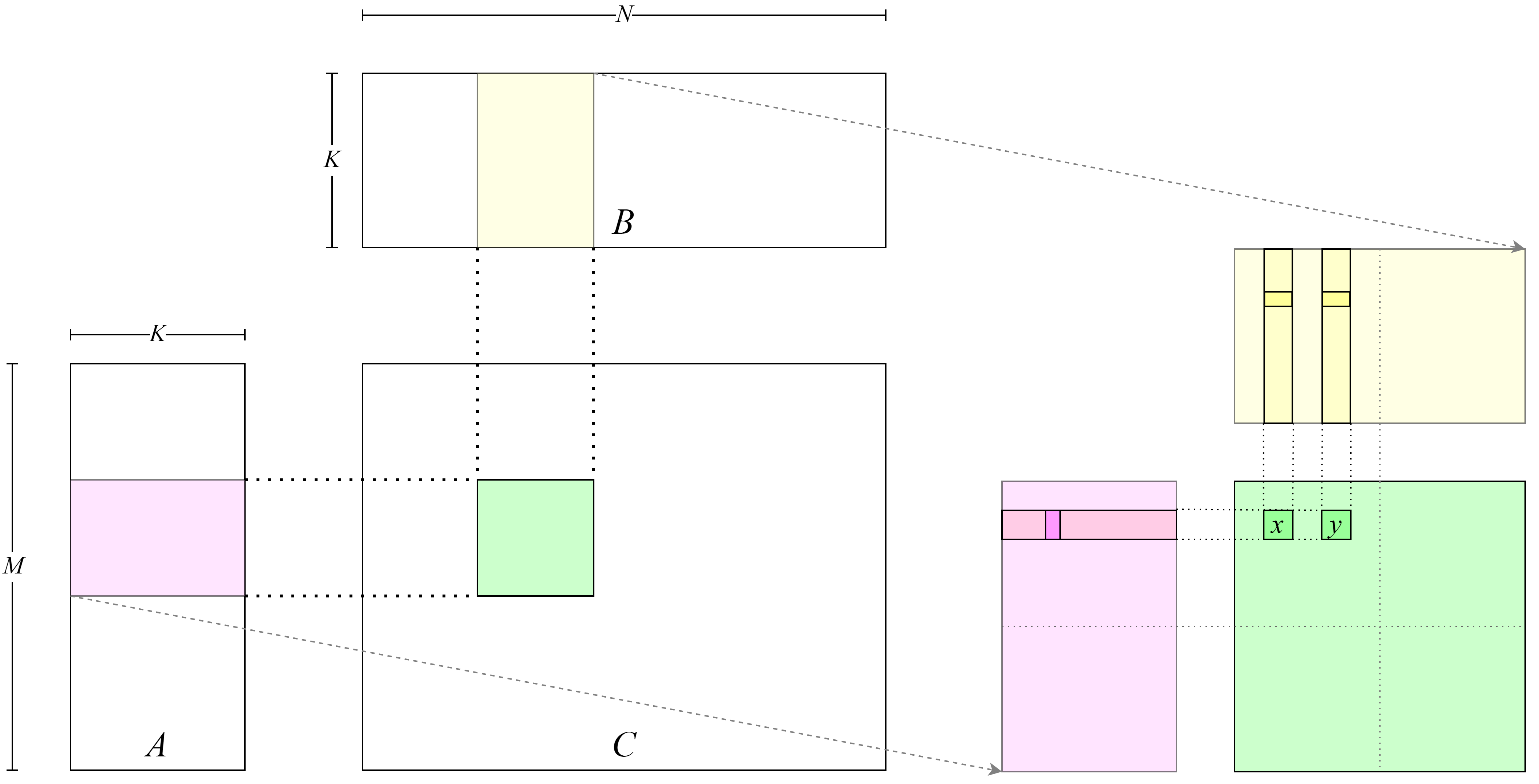
Fig. 7.4.4 Threads loading redundantdata
We have previously mentioned that the inner product can be computed by
loading and accumulating data in \(K\) loops. Specifically, in each
loop, threads that process the same row in matrix \(C\) load the
same data from matrix \(A\), and threads that process the same
column in matrix \(C\) load the same data from matrix \(B\).
However, the code needs to be optimized by dividing \(K\) loops into
\(\frac{K}{tileK}\) outer loops and \(tileK\) inner loops. In
this way, an entire block of data is loaded in each outer loop and
accumulated in each inner loop. Figure :numref:use_smem_store
shows the process of moving data from the global memory to the shared
memory. Before each inner loop starts, the entire tiles in matrix
\(A\) and matrix \(B\) is stored in the shared memory.
Figure :numref:use_smem_load shows the process of moving data from
the shared memory to the register. In each inner loop, data is loaded
from the shared memory and computed. An advantage of this design is that
each thread does not need to load all the data it requires from the
global memory. Instead, the entire thread block loads the data required
for all threads from the global memory and stores the data in the shared
memory. During computational processes, each thread only needs to load
the data it requires from the shared memory.
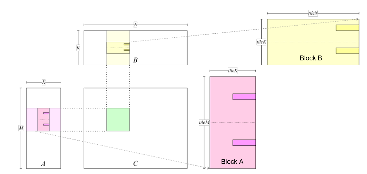
Fig. 7.4.5 Writing data to the sharedmemory
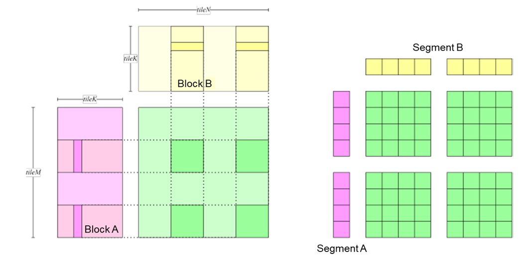
Fig. 7.4.6 Loading data from the sharedmemory
For details about the complete code, see gemm_use_smem.cu.
The test results are as follows:
Max Error: 0.000092
Average Time: 0.617 ms, Average Throughput: 13925.168 GFLOPS
Again, we use Nsight Compute to profile the kernel function and compare
the results with the previous ones. The analysis shows some major
improvements. Specifically, the number of LDG instructions decreases
by 97%, which is consistent with this design. And the value of
SM Utilization increases by 218%, which proves that using the shared
memory can reduce the memory access latency and improve the memory
utilization. Furthermore, the performance of other indicators such as
Pipe Fma Cycles Active also improves significantly, demonstrating
the benefits of the shared memory.
7.4.4. Reducing Register Usage
In previous sections, the data blocks that store matrix \(A\) in the shared memory are arranged in a row-first manner, and the shared memory is loaded by row. We can instead adopt a column-first manner in order to reduce loops and loop variables, thereby reducing the number of registers and improving performance.
For details about the complete code, see gemm_transpose_smem.cu.
The test results are as follows:
Max Error: 0.000092
Average Time: 0.610 ms, Average Throughput: 14083.116 GFLOPS
Analysis by Nsight Compute shows that Occupancy increases by 1.3%.
This is because only 111 registers are used (17 fewer than used by the
previous GPU kernel function). The benefit of reducing the number of
registers varies depending on the GPU architecture. Observations have
shown that the number of STS instructions increases and bank
conflicts occur, meaning that using fewer registers may not have a
positive impact on other GPU architectures.
7.4.5. Hiding Shared Memory Loading Latency
To load data from the shared memory, a GPU uses the LDS instruction.
After issuing this instruction, the GPU will execute the following
instructions without waiting for the data to be loaded to the register
unless the instructions require such data. In the previous section, each
time this instruction is issued during \(tileK\) inner loops, the
mathematical operation that requires the loaded data is performed
immediately. However, the compute unit has to wait for the data to be
loaded from the shared memory, as shown in
Figure :numref:use_smem_pipeline. Accessing the shared memory may
take dozens of clock cycles, but computation instructions can often be
completed within only a few clock cycles. In order to significantly
accelerate memory access, we can hide the shared memory loading latency
by optimizing the pipeline. Specifically, during \(tileK\) inner
loops, loading instructions that prepare data in the next loop can be
loaded at the beginning of each loop, as shown in
Figure :numref:hide_smem_latency. In this way, computation
instructions in the current operation do not require the data in the
next loop. As such, the execution of these computation instructions will
not be blocked by the instructions that load the data for the next loop.
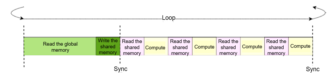
Fig. 7.4.7 Pipeline of the previous GPU kernelfunction
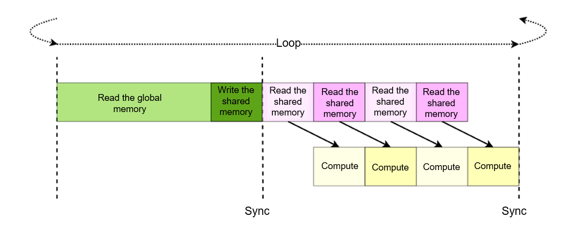
Fig. 7.4.8 Pipeline that hides the shared memory loadinglatency
For details about the complete code, see gemm_hide_smem_latency.cu.
The test results are as follows:
Max Error: 0.000092
Average Time: 0.585 ms, Average Throughput: 14686.179 GFLOPS
Analysis by Nsight Compute shows that the value of
Stall Short Scoreboard decreases by 67% when compared with that of
the previous GPU kernel function. As mentioned before, after GPU memory
load/store instructions are issued, the GPU executes the next
instruction without waiting for the data to be landed in the register.
However, it will set a flag on the Scoreboard and reset the flag after
the data is landed. If instructions that require such data need to be
executed, the GPU will execute them only after the data is landed. The
decrease of Stall Short Scoreboard demonstrates that hiding the
access latency of the shared memory is an effective method to better
utilize the GPU.
7.4.6. Hiding Global Memory Loading Latency
To load data from the global memory, a GPU uses the textttLDG
instruction, the behavior of which is similar to the LDS instruction
used to load data from the shared memory as discussed in the previous
section. At the beginning of each of the \(\frac{K}{tileK}\) outer
loops, instructions that load the data tiles in matrix \(A\) for the
next loop are issued. Because this data is not required by any inner
loop in a given outer loop, the computational processes in the inner
loop will not wait for the read instruction to be completed, thereby
hiding the global memory loading latency. We can also enable data in
buffer to be written to tile in the last loop in the inner loop
after \(tileK - 1\) loops are executed, further reducing the latency
of writing data to tile. Figure :numref:hide_global_latency
shows the optimized pipeline.
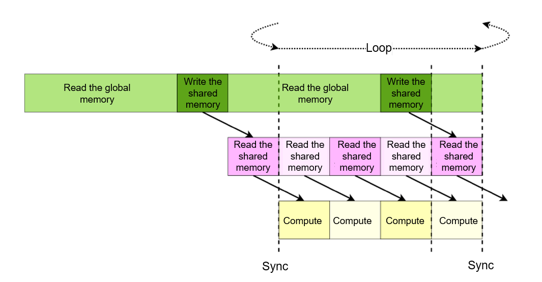
Fig. 7.4.9 Pipeline that hides the global memory loadinglatency
For details about the complete code, see gemm_final.cu.
The test results are as follows:
Max Error: 0.000092
Average Time: 0.542 ms, Average Throughput: 15838.302 GFLOPS
Similar to the Stall Short Scoreboard results obtained in the
previous section, analysis by Nsight Compute shows that the value of
Stall Long Scoreboard (a global memory indicator) decreases by 67%.
Such a significant decrease demonstrates that prefetching data can hide
the global memory to reduce the loading latency.
7.4.7. Performance Optimization Principles
So far, we have discussed various methods to enhance the performance of an accelerator. Even though other methods exist, the principles of performance optimization generally adhere to the following:
Increasing parallelism through resource mapping: Multi-level parallel resources (
blocks,warps, andthreads) are mapped to the data needing computation and transfer to enhance program parallelism.Reducing memory access latency through memory structure optimization: Based on the recognition of data reuse within the same
blockduring computation, the reused data is stored in local memory (like shared memory and registers) to increase locality.Reducing the instruction issue overhead through optimizing instruction execution: The
#pragma unrollfunction is used to unroll loops in order to improve the degree of parallelism at the instruction level and reduce logic judgment. The vectorized load instruction is used to increase bandwidth. For the Ampere architecture, the maximum vectorized load instruction isLDG.E.128, and the data type for data loading isfloat4.Hiding load/store latency by optimizing the memory access pipeline: In instances where the in-memory data undergoes modifications (such as the movement of matrix data), we can optimize the memory access pipeline. This way, the accelerator performs computations during the intervals between data movement, thereby concealing the latency associated with data movement.