8.2. Parallelism Methods

This section explores the prevalent methods for implementing distributed training systems, discussing the design goals and a detailed examination of each parallelism approach.

8.2.1. Classification of Methods

Distributed training amalgamates multiple single-node training systems into a parallel structure to expedite the training process without sacrificing model accuracy. A single-node training system, depicted in Figure Fig. 8.2.1, processes training datasets split into small batches, termed as mini-batches. Here, a mini-batch of data is input into the model, guided by a training program, which generates gradients to enhance model accuracy. Typically, this program executes a deep neural network. To illustrate the execution of a neural network, we employ a computational graph, comprising connected operators. Each operator executes a layer of the neural network, storing parameters to be updated during the training.

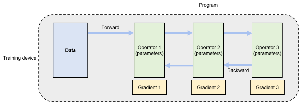
Fig. 8.2.1 Single-node trainingsystem

The execution of a computational graph involves two phases: forward and backward computation. In the forward phase, data is fed into the initial operator, which calculates and generates the data required by the downstream operator. This process is continued sequentially through all operators until the last one concludes its computation. The backward phase initiates from the last operator, computing gradients and updating local parameters accordingly. The process culminates at the first operator. Upon completion of these two phases for a given mini-batch, the system loads the next mini-batch to update the model.

Considering a model training job, partitioning the data and program can facilitate parallel acceleration. Table ch010/ch10-parallel-methods compiles various partition methods. Single-node training systems enable a “single program, single data” paradigm. For parallel computing across multiple devices, data is partitioned and the program is replicated for simultaneous execution, creating a “single program, multiple data” or data parallelism paradigm. Another approach involves partitioning the program, distributing its operators across devices—termed as “multiple programs, single data” or model parallelism. When training exceptionally large AI models, both data and program are partitioned to optimize the degree of parallelism (DOP), yielding a “multiple program, multiple data” or hybrid parallelism paradigm.

:Parallelism methods | Classification | Single Data | Multiple Data | |——————|———————–|——————– | | Single program | single-node execution | data parallelism | | Multiple program | model parallelism | hybrid parallelism |

8.2.2. Data Parallelism

Data parallelism is used when a single node cannot provide sufficient computing power. This is the most common parallelism approach adopted by AI frameworks. Specific implementations include TensorFlow DistributedStrategy, PyTorch Distributed, and Horovod DistributedOptimizer. Given a data-parallel system, assume that the training batch size is \(N\), and that there are \(M\) devices available for parallel acceleration. To achieve data parallelism, the batch size is partitioned into \(M\) partitions, with each device getting \(N/M\) training samples. Sharing a replica of the training program, each device executes and calculates a gradient separately over its own data partition. Each device (indexed \(i\)) calculates a gradient \(G_i\) based on local training samples. To ensure that training program parameters are coherent, local gradients \(G_i\) on different devices are aggregated to calculate an average gradient \((\sum_{i=1}^{N} G_i) / N\). To complete the training on this mini-batch, the training program updates model parameters based on the average gradient.

Figure Fig. 8.2.2 shows a data-parallel training system composed of two devices. For a batch size of 64, each device is assigned 32 training samples and shares the same neural network parameters (or program replicas). The local training samples are passed through the operators in the program replica in sequence for forward and backward computation. During backward computation, the program replicas generate local gradients. Corresponding local gradients on different devices (e.g., gradient 1 on device 1 and gradient 1 on device 2) are aggregated (typically by AllReduce, a collective communication operation) to calculate an average gradient.

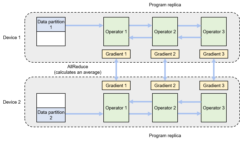
Fig. 8.2.2 Data-parallelsystem

8.2.3. Model Parallelism

Model parallelism is useful when memory constraints make it impossible to train a model on a single device. For example, the memory on a single device will be insufficient for a model that contains a large operator (such as the compute-intensive fully connected layer for classification purpose). In such cases, we can partition this large operator for parallel execution. Assume that the operator has \(P\) parameters and the system consists of \(N\) devices. To minimize the workload on each device given the limited memory capacity, we can evenly assign the parameters across the devices (\(P/N\) = number of parameters per device). This partitioning method is called intra-operator parallelism, which is a typical application of model parallelism.

Figure Fig. 8.2.3 shows an example of intra-operator parallelism implemented by two devices. The neural network in this example consists of two operators. To complete forward and backward computation, operator 1 and operator 2 require 16 GB and 1 GB of memory, respectively. However, in this example, the maximum amount of memory a single device can provide is only 10 GB. To train this network, parallelism is implemented on operator 1. Specifically, the parameters of operator 1 are evenly partitioned into two partitions between device 1 and device 2, meaning that device 1 runs program partition 1 while device 2 runs program partition 2. The network training process starts with feeding a mini-batch of training data to operator 1. Because the parameters of operator 1 are shared between two devices, the data is broadcast to the two devices. Each device completes forward computation based on the local partition of parameters. The local computation results on the devices are aggregated before being sent to downstream operator 2. In backward computation, the data of operator 2 is broadcast to device 1 and device 2, so that each device completes backward computation based on the local partition of operator 1. The local computation results on the devices are aggregated and returned to complete the backward computation process.

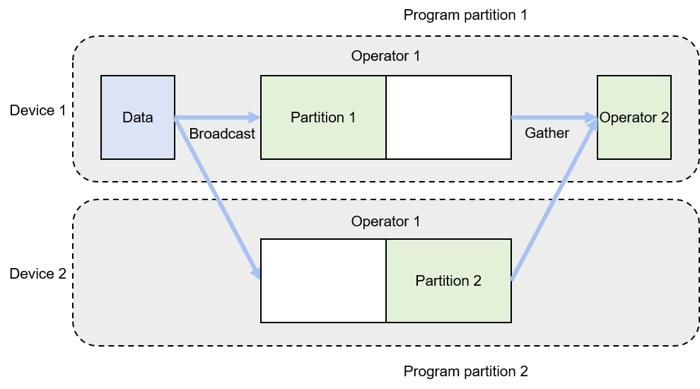
Fig. 8.2.3 Model-parallel system: intra-operatorparallelism

In some cases, the overall model — rather than specific operators — requires more memory than a single device can provide. Given \(N\) operators and \(M\) devices, we can evenly assign the operators across \(M\) devices. As such, each device needs to run forward and backward computation of only \(N/M\) operators, thereby reducing the memory overhead of each device. This application of model parallelism is called inter-operator parallelism.

Figure Fig. 8.2.4 shows an example of inter-operator parallelism implemented by two devices. The neural network in this example has two operators, each requiring 10 GB of memory for computation (20 GB in total). Because the maximum memory a single device can provide in this example is 10 GB, we can place operator 1 on device 1 and operator 2 on device 2. In forward computation, the output of operator 1 is sent to device 2, which uses this output as input to complete forward computation of operator 2. In backward computation, device 2 sends the backward computation result of operator 2 to device 1 for backward computation of operator 1, completing the training on a mini-batch.

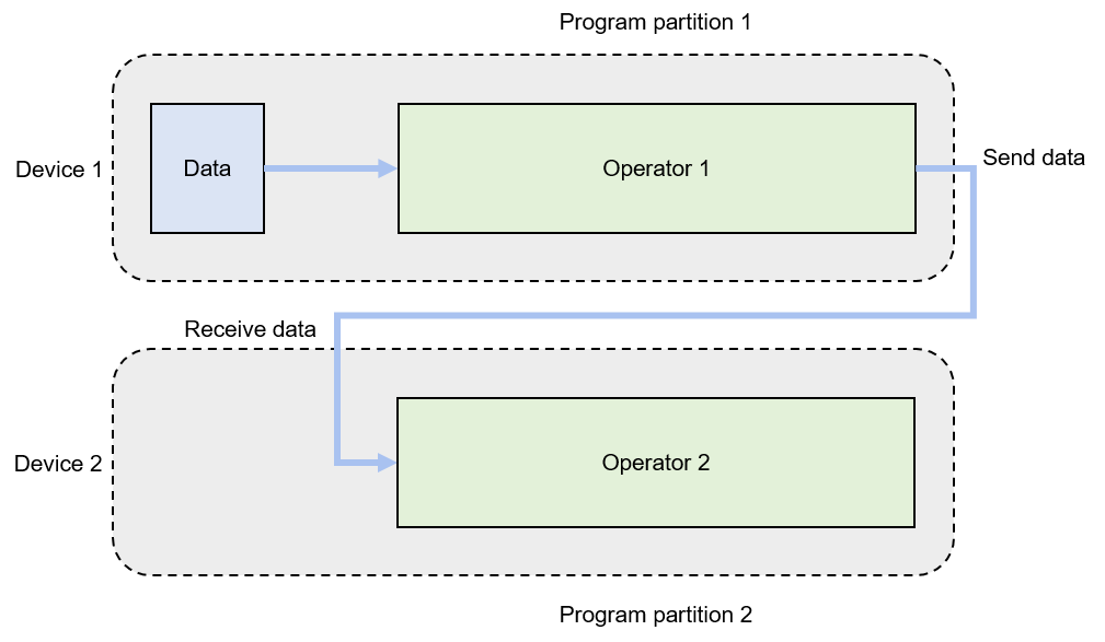
Fig. 8.2.4 Model-parallel system: inter-operatorparallelism

8.2.4. Hybrid Parallelism

In training large AI models, the computing power and memory constraints often go hand in hand. The solution to overcoming these constraints is to adopt a hybrid of data parallelism and model parallelism, that is, hybrid parallelism. Figure Fig. 8.2.5 shows an example of hybrid parallelism implemented by four devices. In this example, inter-operator parallelism is adopted to reduce memory overheads by allocating operator 1 to device 1 and operator 2 to device 2. Device 3 and device 4 are added to the system to achieve data parallelism, thereby improving the computing power of the system. Specifically, the training data is partitioned to data partitions 1 and 2, and the model (consisting of operators 1 and 2) is replicated on devices 3 and 4 respectively. This makes it possible for the program replicas to run in parallel. During forward computation, devices 1 and 3 run the replicas of operator 1 simultaneously and send their respective computation results to devices 2 and 4 to compute the replicas of operator 2. During backward computation, devices 2 and 4 compute gradients simultaneously, and the local gradients are averaged by using the AllReduce operation. The averaged gradient is back-propagated to the replicas of operator 1 on devices 1 and 3, and the backward computation process ends.

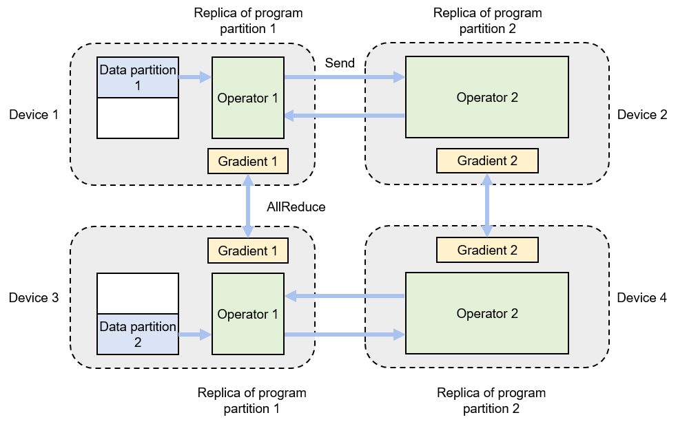
Fig. 8.2.5 Hybrid-parallelsystem