9.3. Model Compression

The previous section briefly described the purpose of model conversion and focused on some common model optimization methods for model deployment. Hardware restrictions differ depending on where models are deployed. For instance, smartphones are more sensitive to the model size, usually supporting models only at the MB level. Larger models need to be compressed using compression techniques before they can be deployed on different computing hardware.

9.3.1. Quantization

Model quantization is a technique that approximates floating-point weights of contiguous values (usually float32 or many possibly discrete values) at the cost of slightly reducing accuracy to a limited number of discrete values (usually int8). As shown in Figure Fig. 9.3.1, \(T\) represents the data range before quantization. In order to reduce the model size, model quantization represents floating-point data with fewer bits. As such, the memory usage during inference can be reduced, and the inference on processors that are good at processing low-precision operations can be accelerated.

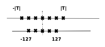
Fig. 9.3.1 Principles ofquantization

The number of bits and the range of data represented by different data types in a computer are different. Based on service requirements, a model may be quantized into models with different number of bits based on service requirements. Generally, single-precision floating-point numbers are used to represent a deep neural network. If signed integers can be used to approximate parameters, the size of the quantized weight parameters may be reduced to a quarter of the original size. Using fewer bits to quantize a model results in a higher compression rate — 8-bit quantization is the mostly used in the industry. The lower limit is 1-bit quantization, which can compress a model to 1/32 of its original size. During inference, efficient XNOR and BitCount bit-wise operations can be used to accelerate the inference.

According to the uniformity of the original ranges represented by the quantized data, quantization can be further divided into linear quantization and non-linear quantization. Because the weights and activations of a deep neural network are usually not uniform in practice, non-linear quantization can theoretically achieve a smaller loss of accuracy. In real-world inference, however, non-linear quantization typically involves higher computation complexity, meaning that linear quantization is more commonly used. The following therefore focuses on the principles of linear quantization.

In Equation (9.3.1), assume that \(r\) represents the floating-point number before quantization. We are then able to obtain the integer \(q\) after quantization.

(9.3.1)\[q=clip(round(\frac{r}{s}+z),q_{min},q_{max})\]

\(clip(\cdot)\) and \(round(\cdot)\) indicate the truncation and rounding operations, and \(q_{min}\) and \(q_{max}\) indicate the minimum and maximum values after quantization, respectively. \(s\) is the quantization interval, and \(z\) is the bias representing the data offset. The quantization is symmetric if the bias (\(z\)) used in the quantization is 0, or asymmetric in other cases. Symmetric quantization reduces the computation complexity during inference because it avoids computation related to \(z\). In contrast, asymmetric quantization determines the minimum and maximum values based on the actual data distribution, and the information about the quantized data is more effectively used. As such, asymmetric quantization reduces the loss of accuracy caused by quantization.

According to the shared range of quantization parameters \(s\) and \(z\), quantization methods may be classified into layer-wise quantization and channel-wise quantization. In the former, separate quantization parameters are defined for each layer. Whereas the latter involves defining separate quantization parameters for each channel. Finer-grained channel-wise quantization yields higher quantization precision, but increases the computation complexity.

Model quantization can also be classified into quantization aware training (QAT) and post-training quantization (PTQ) based on whether training is involved. In QAT, fake-quantization operators are added, and statistics on the input and output ranges before and after quantization are collected during training to improve the accuracy of the quantized model. This method is therefore suitable for scenarios that place strict requirements on accuracy. In PTQ, models are directly quantized after training, requiring only a small amount of calibration data. This method is therefore suitable for scenarios that place strict requirements on usability and have limited training resources.

1. Quantization aware training

QAT simulates quantization during training by including the accuracy loss introduced by fake-quantization operators. In this way, the optimizer can minimize the quantization error during training, leading to higher model accuracy. QAT involves the following steps:

1. Initialization: Set initial values for the \(q_{min}\)/\(q_{max}\) ranges of weights and activations.

2. Building a network for simulated quantization: Insert fake-quantization operators after weights and activations that require quantization.

3. Running QAT: Compute the range (i.e., \(q_{min}\) and \(q_{max}\)) for each weight and activation of the quantized network layer. Then, perform forward computation with the quantization loss considered, so that the loss can be involved in subsequent backpropagation and network parameter update.

4. Exporting the quantized network: Obtain \(q_{min}\) and \(q_{max}\), and compute the quantization parameters \(s\) and \(z\). Substitute the quantization parameters into the quantized formula to transform the network weights into quantized integer values. Then, delete the fake-quantization operators, and add quantization and dequantization operators before and after the quantization network layer, respectively.

2. Post-training quantization

PTQ can be divided into two types: weight quantization and full quantization. Weight quantization quantizes only the weights of a model to compress its size, and then the weights are dequantized to the original float32 format during inference. The subsequent inference process is the same as that of a common float32 model. The advantage of weight quantization is that calibration dataset and quantized operators are not required, and that the accuracy loss is small. However, it does not improve the inference performance, because the operators used during inference are still float32. Full quantization quantizes both the weights and activations of a model, and the quantized operators are executed to accelerate model inference. The quantization of activations requires a small number of calibration datasets (training dataset or inputs of real scenarios) to collect the distribution of the activations at each layer and calibrate the quantized operators. Calibration datasets are used as the input during the quantization of activations. After the inference, the distribution of activations at each layer is collected to obtain quantization parameters. The process is summarized as follows:

1. Use a histogram to represent the distribution \(P_f\) of the original float32 data.

2. Select several \(q_{min}\) and \(q_{max}\) values from a given search space, quantize the activations, and obtain the quantized data \(Q_q\).

3. Use a histogram to represent the distribution of \(Q_q\).

4. Compute the distribution difference between \(Q_q\) and \(P_f\), and find the \(q_{min}\) and \(q_{max}\) values corresponding to the smallest difference between \(Q_q\) and \(P_f\) in order to compute the quantization parameters. Common indicators used to measure the distribution differences include symmetric Kullback-Leibler divergence and Jenson-Shannon divergence.

In addition, the inherent error of quantization requires calibration during quantization. Take the matrix multiplication \(a=\sum_{i=1}^Nw_ix_i+b\) as an example. \(w\) denotes the weight, \(x\) the activation, and \(b\) the bias. To overcome the quantization error, we first calibrate the quantized mean value, and then obtain the mean value of each channel output by the float32 operator and the quantized operator. Assume that the mean value output by the float32 operator of channel \(i\) is \(a_i\), and that output by the quantized operator after dequantization is \(a_{qi}\). From this, we can obtain the final mean value by adding the mean value difference \(a_i-a_q\) of the two channels to the corresponding channel. In this manner, the final mean value is consistent with that output by the float32 operator. We also need to ensure that the distribution after quantization is the same as that before quantization. Assume that the mean value and variance of the weight of a channel are \(E(w_c)\) and \(||w_c-E(w_c)||\), and the mean value and variance after quantization are \(E(\hat{w_c})\) and \(||\hat{w_c}-E(\hat{w_c})||\), respectively. Equation ch-deploy/post-quantization is the calibration of the weight:

(9.3.2)\[\begin{split}\begin{aligned} \hat{w_c}\leftarrow\zeta_c(\hat{w_c}+u_c) \\ u_c=E(w_c)-E(\hat{w_c}) \\ \zeta_c=\frac{||w_c-E(w_c)||}{||\hat{w_c}-E(\hat{w_c})||} \end{aligned} :label: ch-deploy/post-quantization\end{split}\]

As a general model compression method, quantization can significantly improve the memory and compression efficiency of neural networks, and has been widely used.

9.3.2. Model Sparsification

Model sparsification reduces the memory and computation overheads by removing some components (such as weights, feature maps, and convolution kernels) from a neural network. It is a type of strong inductive bias introduced to reduce the computation complexity of the model, just like weight quantization, weight sharing, and pooling.

1. Motivation of model sparsification

Convolution on a convolutional neural network can be considered as a weighted linear combination of the input and the weights of the convolution kernel. In this sense, tiny weights have a relatively small impact on the output. Model sparsification can be justified based on two assumptions:

1. Most neural network models have over-parameterized weights. The number of weight parameters can reach tens or even hundreds of millions.

2. For most computer vision tasks such as detection, classification, and segmentation, useful information accounts for only a small proportion in an activation feature map generated during inference.

As such, model sparsification can be classified into two types according to the source of sparsity: weight sparsification and activation sparsification. Both types reduce the computation workload and model storage requirements by reducing redundant components in a model. In model sparsification, some weak connections are pruned based on the absolute value of weights or activations (i.e. the weight or activation of such connections is set to 0), with the goal of improving the model performance. The sparsity of a model is measured by the proportion of zero-value weights or activation tensors. Because the accuracy of a model typically decreases as its sparsity increases, we hope to minimize such loss when increasing the sparsity.

Neurobiology was the inspiration for inventing neural networks — it has also inspired the sparsification of neural network models. Neurobiologists found that most mammalian brains, including humans, have a process called synapse pruning, which occurs between infancy and adulthood. During synapse pruning, neuron axons and dendrites decay and die off, and the neuron connections are continuously simplified and reconstructed. This process allows brains to work more efficiently and consume less energy.

2. Structured and unstructured sparsification

Let’s first look at weight sparsification. It can be classified into structured and unstructured sparsification. Structured sparsification involves pruning channels or convolution kernels in order to generate regular and smaller weight matrices that are more likely to obtain speedup on CPUs and GPUs. However, this mode is coarse-grained, meaning that it severely reduces the model accuracy.

In contrast, unstructured sparsification allows a weight at any location to be pruned, meaning it is a fine-grained mode that causes less loss to the model accuracy. However, the unstructured mode limits the speedup of sparse models on hardware for a number of reasons:

1. The irregular layout of weights requires many control flow instructions. For instance, the presence of zero values introduces many if-else instructions for decision-making, which inevitably reduces instruction-level parallelism.

2. The computation of convolution kernels is typically multi-threaded. However, the irregular layout of weight matrices on memory causes thread divergence and load imbalance, which therefore affects thread-level parallelism.

3. The irregular layout of weight matrices on the memory hinders data locality and reduces the cache hit rate. Consequently, the load/store efficiency is reduced.

In an attempt to solve these problems, recent work combines structured sparsification with unstructured sparsification. This approach incorporates the advantages of both modes, and overcomes their disadvantages to an extent.

3. Sparsification strategies

Given a neural network model, after deciding to sparsify the weights or activations, we need to determine when and how to perform the sparsification. The most common sparsification process is currently pre-training, pruning, and fine-tuning. With this process, we need to sparsify and fine-tune a converged dense model obtained through training. Given the fact that a pre-trained model contains knowledge it has learned, sparsification on such models will achieve a better effect than directly on the initial model. In addition to pruning the pre-trained model, we usually interleave pruning with network training. Compared with one-shot pruning, iterative pruning is integrated more closely with training, so that redundant convolution kernels can be identified more efficiently. As such, iterative pruning is widely used.

To illustrate how to prune a network, we will use Deep Compression [@han2015deep] as an example. Removing most weights leads to a loss of accuracy of the neural network, as shown in Figure Fig. 9.3.2. Fine-tuning a pruned sparse neural network can help improve model accuracy, and the pruned network may be quantized to represent weights using fewer bits. In addition, using Huffman coding can further reduce the memory cost of the deep neural network.

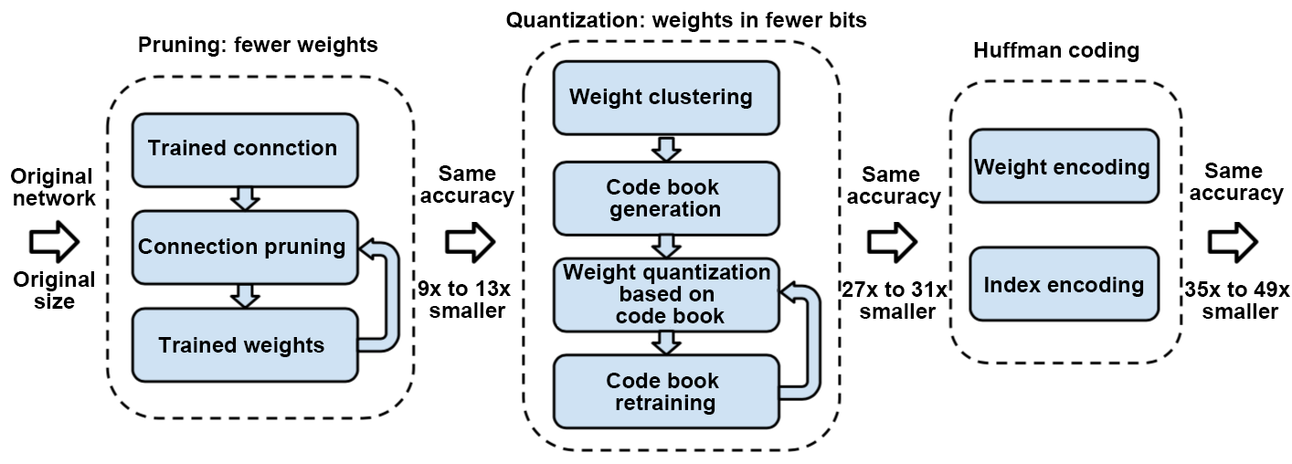
Fig. 9.3.2 Deep Compressionalgorithm

In addition to removing redundant neurons, a dictionary learning-based method can be used to remove unnecessary weights on a deep convolutional neural network. By learning the bases of convolution kernels, the original convolutional kernels can be transformed into the coefficient domain for sparsification. An example of this approach is the work by Bagherinezhad et al. [@bagherinezhad2017lcnn], in which they proposed that the original convolution kernel can be decomposed into a weighted linear combination of the base of the convolution kernel and sparse coefficient.

9.3.3. Knowledge Distillation

Knowledge distillation (KD), also known as the teacher-student learning algorithm, has gained much attention in the industry. Large deep networks tend to deliver good performance in practice, because over-parameterization increases the generalization capability when it comes to new data. In KD, a large pre-trained network serves as the teacher, a deep and thin brand-new neural network serves as the student, supervised by the teacher network. The key to this learning algorithm is how to transfer knowledge converted by the teacher to the student.

Hinton et al. [@Distill] first proposed a teacher-student learning framework. It is used for the learning of deep and thin neural networks by minimizing the differences between the teacher and student neural networks. The teacher network is denoted as \(\mathcal{N}_{T}\) with parameters \(\theta_T\), and the student network is denoted as \(\mathcal{N}_{S}\) with parameters \(\theta_S\). In general, the student network has fewer parameters than the teacher network.

[@Distill] proposed KD, which makes the classification result of the student network more closely resembles the ground truth as well as the classification result of the teacher network, that is, Equation :eqref:c2Fcn:distill.

(9.3.3)\[\mathcal{L}_{KD}(\theta_S) = \mathcal{H}(o_S,\mathbf{y}) +\lambda\mathcal{H}(\tau(o_S),\tau(o_T)),\]

:eqlabel:c2Fcn:distill

where \(\mathcal{H}(\cdot,\cdot)\) is the cross-entropy function, \(o_S\) and \(o_T\) are outputs of the student network and the teacher network, respectively, and \(\mathbf{y}\) is the label. The first item in Equation :eqref:c2Fcn:distill makes the classification result of the student network resemble the expected ground truth, and the second item aims to extract useful information from the teacher network and transfer the information to the student network, \(\lambda\) is a weight parameter used to balance two objective functions, and \(\tau(\cdot)\) is a soften function that smooths the network output.

Equation :eqref:c2Fcn:distill only extracts useful information from the output of the teacher network classifier — it does not mine information from other intermediate layers of the teacher network. Romero et al. [@FitNet] proposed an algorithm for transferring useful information from any layer of a teacher network to a small student network. Note that not all inputs are useful for convolutional neural network computing and subsequent task execution. For example, in an image containing an animal, it is important to classify and identify the region where the animal is rather than the background information. Therefore, it is an efficient way to select useful information from the teacher network. Zagoruyko and Komodakis [@attentionTS] proposed a learning method based on an attention loss function to improve the performance of the student network. This method introduces an attention module. The attention module generates an attention map, which identifies the importance of different areas of an input image to the classification result. The attention map is then transferred from the teacher network to the student network, as depicted in Figure  ch-deploy/attentionTS.

KD is an effective method to optimize small networks. It can be combined with other compression methods such as pruning and quantization to train efficient models with higher accuracy and less computation workload.

Teacher-student neural network learning algorithm