5.4. Automatic Differentiation

In the following, we describe the key methodologies applied in automatic differentiation.

5.4.1. Types of Differentiation Methods

Differentiation constitutes a collection of methodologies enabling the efficient and precise evaluation of derivatives within computer programs. Since the 1960s and 1970s, it has been extensively utilized across multiple sectors including fluid mechanics, astronomy, and mathematical finance . Its theories and implementation have been rigorously studied over time.

With the advancement of deep learning, which has shown remarkable progress across an expanding range of machine learning tasks in recent years, automatic differentiation has found wide-spread application in the field of machine learning. Given that many optimization algorithms employed in machine learning models necessitate derivatives of the models, automatic differentiation has emerged as an integral component within mainstream machine learning frameworks such as TensorFlow and PyTorch.

There are four primary methods to evaluate derivatives in computer programs, each of which is explained in the following sections.

5.4.1.1. Manual Differentiation

Manual differentiation involves the direct computation of the derivative expression of a function, a task which hinges upon the input values specified within a program. Although this method could seem appealing due to its simplicity and directness, it is worth noting that it comes with its share of limitations.

A primary drawback of manual differentiation is the need to re-derive and re-implement the derivative every time a function changes, which can be laborious and time-consuming. This is especially true for complex functions or when working on large-scale projects where the function might undergo frequent updates.

Moreover, manual differentiation can be prone to human errors. The process of deriving complex functions often involves intricate chains of mathematical reasoning. A slight oversight or error in any of these steps can lead to an incorrect derivative, which, in turn, can greatly affect the outcome of the computation. This susceptibility to mistakes can add a layer of uncertainty to the reliability of this method.

Furthermore, in cases where high-order derivatives or partial derivatives with respect to many variables are needed, manual differentiation quickly becomes unfeasible due to the increase in complexity. The difficulty of computing these derivatives correctly grows exponentially with the number of variables and the order of the derivative.

5.4.1.2. Numerical Differentiation

Numerical differentiation is an approach that logically stems from the fundamental definition of a derivative and employs the method of difference approximation. The basic formula for numerical differentiation can be described as follows:

(5.4.1)\[f^{'}(x)=\lim_{h \to 0}\frac{f(x+h)-f(x)}{h}\]

In this equation, for a sufficiently small value of the step size \(h\), the difference quotient \(\frac{f(x+h)-f(x)}{h}\) is used as an approximation of the derivative. The inherent error in this approximation is referred to as the truncation error, which theoretically diminishes as the value of \(h\) approaches zero. This suggests that a smaller step size would yield a more accurate approximation.

However, the scenario in practice is not always so straightforward due to the phenomenon of round-off error. This error arises from the finite precision of floating-point arithmetic operations in digital computer systems. As the value of \(h\) decreases, the round-off error conversely increases, adding a degree of uncertainty to the computation.

This creates a complex interplay between truncation error and round-off error. When the value of \(h\) is large, the truncation error dominates, whereas when \(h\) is small, the round-off error is more significant. Consequently, the total error of numerical differentiation achieves a minimum at an optimal \(h\) value that balances these two types of errors.

In a nutshell, while numerical differentiation offers the advantage of relative simplicity in implementation, it suffers from certain limitations with regard to accuracy. The complexities arising from the interplay between truncation and round-off errors make it less reliable for certain tasks, particularly when high precision is required. Therefore, for many practical applications, more sophisticated techniques of automatic differentiation are preferred.

5.4.1.3. Symbolic Differentiation

Symbolic differentiation involves the use of computer programs to automatically calculate derivatives. This is accomplished by recursively transforming function expressions in accordance with specific differentiation rules. These rules can be summarized as follows:

(5.4.2)\[\frac{\partial}{\partial x}(f(x)+g(x))\rightsquigarrow\frac{\partial}{\partial x}f(x)+\frac{\partial }{\partial x}g(x)\]

(5.4.3)\[\frac{\partial}{\partial x}(f(x)g(x))\rightsquigarrow(\frac{\partial}{\partial x}f(x))g(x)+f(x)(\frac{\partial}{\partial x}g(x))\]

Symbolic differentiation has been integrated into many modern algebraic systems such as Mathematica, as well as machine learning frameworks like Theano. It successfully addresses the issues related to hard-coding derivatives inherent in manual differentiation, thus automating the differentiation process and minimizing human error.

Despite these advantages, symbolic differentiation has its own set of challenges. One of its primary limitations is its strict adherence to transforming and expanding expressions recursively, without the ability to reuse previous results of transformations. This can lead to a phenomenon known as expression swell , which results in highly complex and expanded expressions that can significantly slow down computation and increase memory usage.

In addition, symbolic differentiation requires that the expressions to be differentiated are defined in closed form. This constraint largely restricts the use of control flow statements such as loops and conditional branches, which are common in programming. This lack of flexibility can significantly limit the design and expressivity of neural networks within machine learning frameworks, as these often require intricate control flow structures for more advanced operations.

5.4.1.4. Automatic Differentiation

Automatic differentiation cleverly amalgamates the strategies of numerical differentiation and symbolic differentiation to offer an efficient and precise mechanism for derivative evaluation. It breaks down the arithmetic operations in a program into a finite set of elementary operations, for each of which the rules of derivative evaluation are already known. Upon determining the derivative of each elementary operation, the chain rule is applied to synthesize these individual results, ultimately yielding the derivative of the entire program.

The fundamental strength of automatic differentiation lies in its ability to sidestep the primary drawbacks of both numerical and symbolic differentiation. Unlike numerical differentiation, which suffers from precision issues due to truncation and round-off errors, automatic differentiation facilitates accurate derivative evaluations. Furthermore, it mitigates the issue of expression swell, a significant concern in symbolic differentiation, by decomposing the program into a series of elementary expressions. Symbolic differentiation rules are only applied to these simplified expressions, and the derivative results are reused to enhance efficiency.

Automatic differentiation also surpasses symbolic differentiation in its capability to handle control flow statements. It has the ability to process branching, looping, and recursion, enhancing its flexibility and applicability to complex computational scenarios.

In contemporary applications, automatic differentiation has found widespread use in deep learning frameworks for the evaluation of derivatives, given its blend of accuracy and efficiency. The subsequent sections delve into the mechanics and implementation aspects of automatic differentiation, elucidating its role as a crucial tool in computational mathematics and machine learning.

5.4.2. Forward Mode and Reverse Mode

Automatic differentiation can be categorized into two modes, forward and reverse, based on the sequence in which the chain rule is applied. Consider a composite function \(y=a(b(c(x)))\). The formula to calculate its gradient, \(\frac{\partial y}{\partial x}\), is given as:

(5.4.4)\[\frac{\partial y}{\partial x}=\frac{\partial y}{\partial a}\frac{\partial a}{\partial b}\frac{\partial b}{\partial c}\frac{\partial c}{\partial x}\]

In the forward mode of automatic differentiation, the computation of the gradient originates from the inputs, as shown in the following formulation:

(5.4.5)\[\frac{\partial y}{\partial x}=(\frac{\partial y}{\partial a}(\frac{\partial a}{\partial b}(\frac{\partial b}{\partial c}\frac{\partial c}{\partial x})))\]

Conversely, in the reverse mode, the computation of the gradient begins from the outputs, represented by the equation:

(5.4.6)\[\frac{\partial y}{\partial x}=(((\frac{\partial y}{\partial a}\frac{\partial a}{\partial b})\frac{\partial b}{\partial c})\frac{\partial c}{\partial x})\]

To illustrate the computation methods of the two modes, let us consider the following function and aim to evaluate its derivative, \(\frac{\partial y}{\partial x_1}\) at the point \((x_1, x_2)=(2,5)\):

(5.4.7)\[y=f(x_1,x_2)=ln(x_1)+{x_1}{x_2}-sin(x_2)\]

Figure :numref:ch04/ch04-calculation_graph represents the computational graph of this function, providing a visual demonstration of how automatic differentiation processes the function in both forward and reverse modes. This distinction between forward and reverse modes is particularly important when dealing with functions of multiple variables, with each mode having specific use cases and efficiency implications.

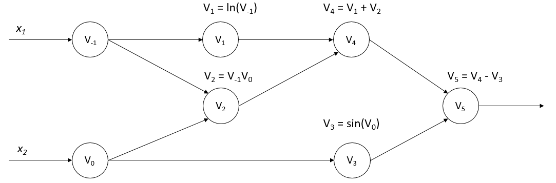
Fig. 5.4.1 Computational graph of the examplefunction

5.4.2.1. Forward Mode

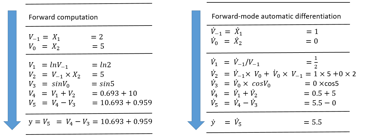
Fig. 5.4.2 Illustration of forward-mode automaticdifferentiation

Figure :numref:ch04/ch04-forward-mode-compute-function elucidates thecomputation process within the forward mode. The sequence of elementaryoperations, derived from the source program, is displayed on the left.Following the chain rule and using established derivative evaluationrules, we sequentially compute each intermediate variable \({\dot{v}_i}=\frac{\partial v_i}{\partial x_1}\) from top to bottom, as depicted on the right. Consequently, this leads to the computation ofthe final variable \({\dot{v}_5}=\frac{\partial y}{\partial x_1}\). In the process of derivative evaluation of a function, we obtain a setof partial derivatives of any output with respect to any input of thisfunction. For a function \(f:{\mathbf{R}^n}\to \mathbf{R}^m\), where \(n\) is the number of independent input variables \(x_i\), and \(m\) is thenumber of independent output variables \(y_i\), the derivative resultscorrespond to the following Jacobian matrix:

(5.4.8)\[\begin{split}\mathbf{J}_{f}= \begin{bmatrix} \frac{\partial y_1}{\partial x_1} & \cdots & \frac{\partial y_1}{\partial x_n} \\ \vdots & \ddots & \vdots \\ \frac{\partial y_m}{\partial x_1} & \cdots & \frac{\partial y_m}{\partial x_n} \end{bmatrix}\end{split}\]

Each forward pass of function \(f\) results in partial derivatives of alloutputs with respect to a single input, represented by the vectorsbelow. This corresponds to one column of the Jacobian matrix. Therefore,executing \(n\) forward passes gives us the full Jacobian matrix.

(5.4.9)\[\begin{split}\begin{bmatrix} \frac{\partial y_1}{\partial x_i} \\ \vdots \\ \frac{\partial y_m}{\partial x_i} \end{bmatrix}\end{split}\]

The forward mode allows us to compute Jacobian-vector products byinitializing \(\dot{\mathbf{x}}=\mathbf{r}\) to generate the results for asingle column. As the derivative evaluation rules for elementaryoperations are pre-determined, we know the Jacobian matrix for all theelementary operations. Consequently, by leveraging the chain rule toevaluate the derivatives of \(f\) propagated from inputs to outputs, wesecure one column in the Jacobian matrix of the entire network.

(5.4.10)\[\begin{split}\mathbf{J}_{f}\mathbf{r}= \begin{bmatrix} \frac{\partial y_1}{\partial x_1} & \cdots & \frac{\partial y_1}{\partial x_n} \\ \vdots & \ddots & \vdots \\ \frac{\partial y_m}{\partial x_1} & \cdots & \frac{\partial y_m}{\partial x_n} \end{bmatrix} \begin{bmatrix} r_1 \\ \vdots \\ r_n \end{bmatrix}\end{split}\]

5.4.2.2. Reverse Mode

Figure :numref:ch04/ch04-backward-mode-compute illustrates theautomatic differentiation process in the reverse mode. The sequence ofelementary operations, derived from the source program, is displayed onthe left. Beginning from \(\bar{v}_5=\bar{y}=\frac{\partial y}{\partial y}=1\), we sequentiallycompute each intermediate variable \({\bar{v}_i}=\frac{\partial y_j}{\partial v_i}\) from bottom to top, leveraging the chain rule and established derivative evaluation rules (as depicted on the right). Thus, we can compute the final variables \({\bar{x}_1}=\frac{\partial y}{\partial x_1}\) and \({\bar{x}_2}=\frac{\partial y}{\partial x_2}\).

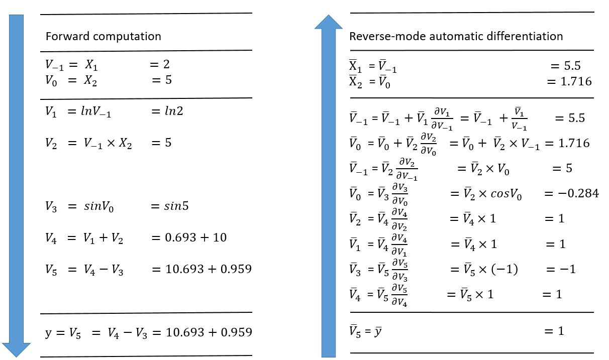
Fig. 5.4.3 Illustration of reverse-mode automaticdifferentiation

Every reverse pass of function \(f\) produces partial derivatives of asingle output with respect to all inputs, represented by the followingvectors. This corresponds to a single row of the Jacobian matrix.Consequently, executing \(m\) reverse passes gives us the full Jacobianmatrix.

(5.4.11)\[\begin{bmatrix} \frac{\partial y_j}{\partial x_1} & \cdots & \frac{\partial y_j}{\partial x_n} \end{bmatrix}\]

Similarly, we can compute vector-Jacobian products to obtain the resultsfor a single row.

(5.4.12)\[\begin{split}\mathbf{r}^{T}\mathbf{J}_{f}= \begin{bmatrix} r_1 & \cdots & r_m \end{bmatrix} \begin{bmatrix} \frac{\partial y_1}{\partial x_1} & \cdots & \frac{\partial y_1}{\partial x_n} \\ \vdots & \ddots & \vdots \\ \frac{\partial y_m}{\partial x_1} & \cdots & \frac{\partial y_m}{\partial x_n} \end{bmatrix}\end{split}\]

The quantity of columns and rows in a Jacobian matrix directly influences the number of forward and reverse passes needed to solve it for a given function \(f\). This characteristic is particularly significant when determining the most efficient method of automatic differentiation.

When the function has significantly fewer inputs than outputs \((f:{\mathbf{R}^n}\to \mathbf{R}^m, n << m)\), the forward mode proves to be more efficient. Conversely, when the function has considerably more inputs than outputs \((f:{\mathbf{R}^n}\to \mathbf{R}^m, n >> m)\), the reverse mode becomes advantageous.

For an extreme case where the function maps from \(n\) inputs to a single output \(f:{\mathbf{R}^n}\to \mathbf{R}\), we can evaluate all the derivatives of the output with respect to the inputs \((\frac{\partial y}{\partial x_1},\cdots,\frac{\partial y}{\partial n})\) using a single reverse pass or \(n\) forward passes. This is a situation akin to derivative evaluation for a multi-input, single-output network, a structure frequently encountered in machine learning.

Due to this feature, reverse-mode automatic differentiation forms the basis for the backpropagation algorithm, a key technique for training neural networks. By enabling efficient computation of gradients, especially in scenarios with high-dimensional input data and scalar output (common in many machine learning applications), reverse-mode automatic differentiation has become indispensable in the field.

However, the reverse mode does come with certain limitations. For instance, once a source program is decomposed into a sequence of elementary operations in the forward mode, inputs can be obtained synchronously during the execution of these operations. This is possible because the sequence of derivative evaluations aligns with the sequence of operation execution. In contrast, in the reverse mode, the sequence for derivative evaluation is the inverse of the execution sequence of the source program, leading to a two-phased computation process. The initial phase entails executing the source program and storing the intermediate results in memory, while the subsequent phase involves retrieving these intermediate results to evaluate the derivatives. Due to the additional steps involved, the reverse mode requires more memory.

5.4.3. Implementing Automatic Differentiation

This section explores typical design patterns for implementing automatic differentiation in machine learning frameworks. These design patterns can be broadly classified into three categories: elemental libraries, operator overloading, and source transformation.

5.4.3.1. Elemental Libraries

Elemental libraries encapsulate elementary expressions and their differential expressions as library functions. When coding, users must manually decompose a program into a set of elementary expressions and replace them with corresponding library functions. Take the program \(a=(x+y)/z\) as an example; it needs to be manually decomposed as follows:

t = x + y
    a = t / z

Subsequently, users replace the decomposed elementary expressions with appropriate library functions:

// The parameters include variables x, y, and t and their derivative variables dx, dy, and dt.
    call ADAdd(x, dx, y, dy, t, dt)
    // The parameters include variables t, z, and a and their derivative variables dt, dz, and da.
    call ADDiv(t, dt, z, dz, a, da)

The library functions, ADAdd and ADDiv, use the chain rule to define the Add and Div differential expressions, respectively. This is illustrated in Code lst:diff.

lst:diff

def ADAdd(x, dx, y, dy, z, dz):
    z = x + y
    dz = dy + dx

    def ADDiv(x, dx, y, dy, z, dz):
    z = x / y
    dz = dx / y + (x / (y * y)) * dy

Elemental libraries constitute a simple and straightforward way of implementing automatic differentiation for programming languages. However, this approach requires users to manually decompose a program into elementary expressions before calling library functions for programming. Furthermore, it is not possible to use the native expressions found in programming languages.

5.4.3.2. Operator Overloading

Leveraging the polymorphism characteristic inherent in modern programming languages, the Operator Overloading design pattern redefines the semantics of elementary operations and successfully encapsulates their differentiation rules. During the execution phase, it methodically documents the type, inputs, and outputs of every elementary operation within a data structure known as a ‘tape’. These tapes have the ability to generate a trace, serving as a pathway for applying the chain rule. This makes it possible to aggregate elementary operations either in a forward or backward direction to facilitate differentiation. As depicted in Code lst:OO, we utilize the AutoDiff code from automatic differentiation libraries as a case in point to overload the basic arithmetic operators in programming languages.

lst:OO

namespace AutoDiff
    {
        public abstract class Term
        {
            // To overload and call operators (`+`, `*`, and `/`),
            // TermBuilder records the types, inputs, and outputs of operations in tapes.
            public static Term operator+(Term left, Term right)
            {
                return TermBuilder.Sum(left, right);
            }
            public static Term operator*(Term left, Term right)
            {
                return TermBuilder.Product(left, right);
            }
            public static Term operator/(Term numerator, Term denominator)
            {
                return TermBuilder.Product(numerator, TermBuilder.Power(denominator, -1));
            }
        }

        // Tape data structures include the following basic elements:
        // 1) Arithmetic results of operations
        // 2) Derivative evaluation results corresponding to arithmetic results of operations
        // 3) Inputs of operations
        // In addition, functions Eval and Diff are used to define the computation and differentiation rules of the arithmetic operations.
        internal abstract class TapeElement
        {
            public double Value;
            public double Adjoint;
            public InputEdges Inputs;

            public abstract void Eval();
            public abstract void Diff();
        }
    }

Operator overloading carries the advantage of tracing the program through function calls and control flows, resulting in an implementation process that is both simple and straightforward. However, the requirement to trace the program during runtime introduces certain challenges. Specifically, operator overloading is necessitated to execute reverse-mode differentiation along the trace, which can potentially cause a drop in performance, particularly for elementary operations that are executed swiftly. Furthermore, due to the constraints of runtime, operator overloading is unable to conduct compile-time graph optimization prior to execution, and the unfolding of control flows must be based on the information available at runtime. Despite these challenges, operator overloading is extensively employed in the PyTorch framework for automatic differentiation due to its inherent simplicity and adaptability.

5.4.3.3. Source Transformation

Source transformation is a design pattern that enriches programming languages and scrutinizes a program’s source code or its Abstract Syntax Tree (AST) to automatically deconstruct the program into a set of differentiable elementary operations, each with predefined differentiation rules. The chain rule is then employed to amalgamate the differential expressions of the elementary operations, resulting in a novel program expression that conducts the differentiation. Source Transformation is integral to machine learning frameworks such as TensorFlow and MindSpore.

Unlike operator overloading, which functions within programming languages, source transformation necessitates parsers and tools that manipulate IRs. It also requires transformation rules for function calls and control flow statements, such as loops and conditions. The principal advantage of source transformation is that the automatic differentiation transformation occurs only once per program, thus eliminating runtime overhead. Additionally, the complete differentiation program is available during compilation, enabling ahead-of-time optimization using compilers.

However, source transformation presents a higher implementation complexity compared to the other approaches. It must support a wider array of data types and operations, and it necessitates preprocessors, compilers, or interpreters of extended languages, along with a more robust type-checking system. Even though source transformation does not manage automatic differentiation transformation at runtime, it still must ensure that certain intermediate variables from the forward pass are accessible by the adjoint in reverse mode. Two modes are available to facilitate this:

• Tape-based mode: This mode requires a global tape that ensures the accessibility of intermediate variables. In this method, the primitive function is augmented so that intermediate variables are written to functions in the tape during the forward pass, and the adjoint program reads these intermediate variables from the tape during the backward pass. The tape used in source transformation primarily stores the intermediate variables, while the tape used in operator overloading additionally stores the executed operation types. Given that the tape is a data structure constructed at runtime, custom compiler optimizations are required. Moreover, tape read and write operations must be differentiable to support higher-order differentiation, which involves multiple applications of reverse mode. As most tape-based tools do not differentiate tape read and write operations, such tools do not support reverse-over-reverse automatic differentiation.

• Closure-based mode: This mode was proposed to mitigate some of the limitations observed in the tape-based mode. Within functional programming, closures can capture the execution environment of a statement and identify the non-local use of intermediate variables.