8.3. Pipeline Parallelism with Micro-Batching

In addition to data parallelism and model parallelism, pipeline parallelism is another common method for distributed training. Pipeline parallelism is often used in large-scale model-parallel systems that are designed to overcome the memory shortage in individual devices through intra- and inter-operator parallelism. However, when such systems are running, downstream devices in the computational graph remain idle for a long time — they cannot perform computation until it is completed in upstream devices. Consequently, the average utilization of devices is low. This phenomenon is known as model parallelism bubbles.

To reduce bubbles, we can build pipelines in training systems. Essentially, this approach divides each mini-batch in the training data into multiple micro-batches. For example, if a mini-batch with \(D\) training samples is divided into \(M\) micro-batches, then each micro-batch has \(D/M\) data samples. These micro-batches enter the training system in sequence and go through forward and backward computation. In this way, the system computes a gradient of each micro-batch, and then caches the gradient. After the preceding steps are completed for all micro-batches, the cached gradients are summed to compute the average gradient (equivalent to the gradient of the entire mini-batch) based on which the model parameters are updated.

Figure Fig. 8.3.1 shows an execution example of a pipeline training system. In this example, model parameters are split among four devices for storage. To fully utilize the four devices, the mini-batch is divided into two micro-batches. It is assumed that \(F_{i,j}\) represents the \(i\)th forward computation task of the \(j\)th micro-batch, and \(B_{i,j}\) represents the \(i\)th backward computation task of the \(j\)th micro-batch. After completing the forward computation of the first micro-batch (denoted as \(F_{0,0}\)), device 1 sends the intermediate result to device 2, which then starts the corresponding forward computation task (denoted as \(F_{1,0}\)). At the same time, device 1 starts the forward computation task of the second micro-batch (denoted as \(F_{0,1}\)). Forward computation will be finally completed on the last device in the pipeline, that is, device 3.

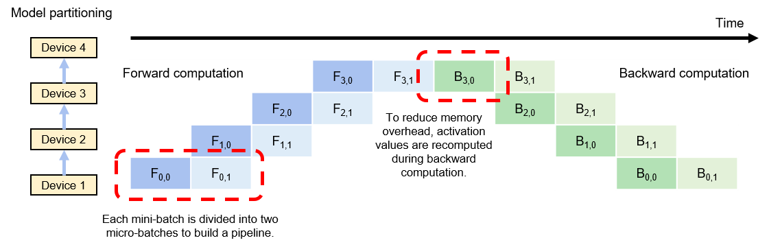
Fig. 8.3.1 Pipeline-parallelsystem

The system then starts backward computation: Device 4 starts the backward computation task of the first micro-batch (denoted as \(B_{3,0}\)). On completion, the intermediate result is sent to device 3, which then starts the corresponding backward computation task (denoted as \(B_{2,0}\)). At the same time, device 4 caches the gradient of the first micro-batch and starts computation for the second micro-batch (denoted as \(B_{3,1}\)). When device 4 completes all backward computation, it sums the locally cached gradients and then divides the sum by the number of micro-batches to compute the average gradient. This gradient is used to update model parameters.

It should be noted that gradient computation often needs the activation values generated in forward computation. In classical model-parallel systems, activation values are cached in memory and directly used during backward computation to avoid repeated computation. In pipeline training systems, however, these values are not cached due to the strain on memory resources. Instead, they are recomputed during backward computation.

For optimal performance of pipeline training systems, the sizes of micro-batches need to be debugged. Upon completion of forward computation tasks, devices have to wait until all backward computation tasks start, meaning that the devices remain idle during this period. As shown in Figure Fig. 8.3.1, after completing the two forward computation tasks, device 1 waits for an extended period of time before it can start the two backward computation tasks. This waiting time is referred to as pipeline bubbles. To minimize pipeline bubbles, a common practice is to increase the number of micro-batches to the maximum extent so that backward computation can start as early as possible. However, this practice may result in each micro-batch containing insufficient training samples, failing to fully utilize the massive computing cores in hardware accelerators. Therefore, the optimal number of micro-batches is jointly determined by a plurality of factors (such as pipeline depth, micro-batch size, and quantity of computing cores in an accelerator).

8.3.1. Expert Parallelism

Mixture of Experts (MoE) models have gained significant popularity due to their ability to effectively scale the size of models. Traditional neural networks typically require a linear increase in computational resources as the number of parameters grows, making extremely large networks prohibitively expensive to train. MoE models address this challenge by specializing different parts of the model—referred to as experts—to handle specific subsets of the data or tasks, thereby enabling a more efficient use of computational resources.

MoE models achieve this specialization by dynamically selecting which experts to activate for a given input. This approach allows the model to scale to billions of parameters without a proportional increase in computational demand during inference. In other words, the demand for computational resources grows sub-linearly with the number of parameters. This efficiency makes MoE models particularly attractive for applications that require both high capacity and scalability, such as natural language processing and recommendation systems.

An MoE model consists of the following key components: (i) Experts: These are individual neural network sub-models, each trained to handle different aspects or subsets of the data. For example, in a language model, one expert might specialize in syntax while another focuses on semantics, (ii) Gating Network: This component determines which experts to activate for a given input. The gating network takes the input data and outputs a set of weights or selections that decide the contribution of each expert to the final output, and (iii) Aggregation Mechanism: After the experts process the input, their outputs are combined (aggregated) to produce the final result. The aggregation is typically weighted by the gating network’s output, allowing the model to emphasize the contributions of the most relevant experts.

To parallelize an MoE model, the expert parallelism strategy will follow several key steps: (i)