6.4. Memory Allocation
Memory allocation is a crucial aspect of conventional computer memory hierarchy, acting as a link between cache and disk storage. It provides more storage capacity than the cache and enables faster access compared to disk storage. With the progress of deep learning, accommodating large deep neural networks within the memory of hardware accelerators or AI processors has become increasingly challenging. To overcome this obstacle, various solutions have been developed, including memory reuse, contiguous memory allocation, and in-place memory allocation. Proper implementation of contiguous memory allocation and in-place memory allocation can enhance the execution efficiency of operators and further optimize performance.
6.4.1. Device Memory
In a deep learning architecture, the memory closest to the hardware accelerator (such as the GPU or AI processor) is usually referred to as the device memory, and that closest to the CPU is referred to as the host memory. As shown in Figure Fig. 6.4.1, the CPU can directly access the host memory but not the device memory. Similarly, the AI processor can directly access the device memory but not the host memory. In a typical network training process, data needs to be loaded from disk storage to the host memory, where it is then processed. After that, the data is copied from the host memory to the device memory, so that the device can directly access the data. When the computation is finished, the user can obtain the training result once the result data is copied from the device memory back to the host memory.
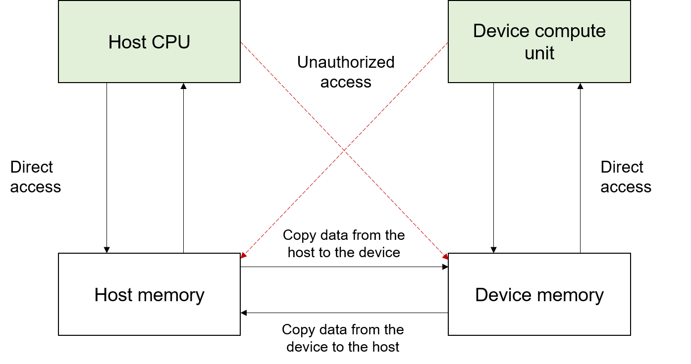
Fig. 6.4.1 Host memory and devicememory
6.4.2. Process of Memory Allocation
The memory allocation module allocates device memory to the input and
output of each operator in a graph. The compiler frontend interprets the
user script into an IR, based on which the compiler backend performs
operator selection and optimization to determine information such as the
shape, data type, and format of each input/output tensor of each
operator. With this information, the size of each input/output tensor of
each operator can be calculated using Equation
ch05/equation-04:
:eqlabel:equation:ch05/equation-04
Unaligned memory access can be time-consuming, because the transfer of data to and from memory is most efficient in chunks of 4, 8, or 16 bytes. When the size of the data to be transferred is not a multiple of any of these sizes, one or more empty bytes are padded to align the data in memory.
Figure Fig. 6.4.2 illustrates an example of memory allocation.
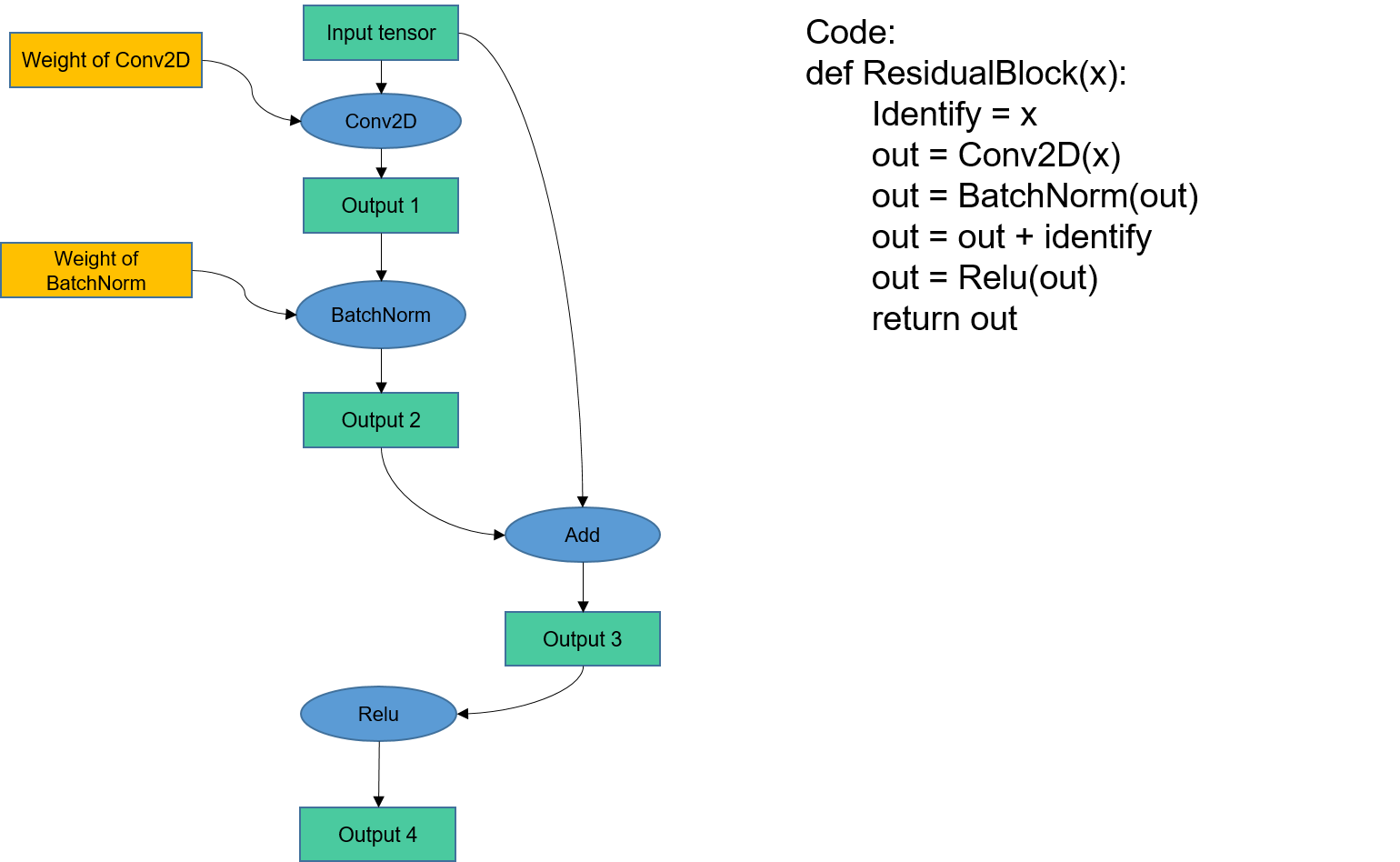
Fig. 6.4.2 Memory allocationexample
In this example, memory addresses are assigned to the input tensor, Conv2D’s weight, and Conv2D’s output. Subsequently, a memory address is allocated to the input of BatchNorm. Since the input of BatchNorm is the same as the output of Conv2D, which already has a allocated memory address, the output address of Conv2D can be shared with the input of BatchNorm. This approach avoids redundant memory allocation and unnecessary memory copies. The entire training process in this example involves allocating memory for three types based on their data lifetime: the initial input of the graph, the weights or attributes of operators, and the output tensor of the final operator.
Frequent allocations and deallocations of memory blocks of various sizes
using functions like malloc can significantly degrade performance.
To mitigate this issue, memory pools can be employed. Memory pools
involve pre-allocating a specific amount of memory, allowing memory
blocks to be dynamically allocated from the pool as needed and returned
for reuse.
Memory pools are widely utilized in AI frameworks to manage frequent allocations of device memory and ensure consistent memory lifetime for tensors. Different AI frameworks adopt similar memory pool designs. Figure Fig. 6.4.3 presents an example of memory allocation in an AI framework. In this case, each tensor’s memory is allocated from a pre-allocated device memory space using double pointers to offset the start and end addresses. Weight tensors of operators are allocated memory by offsetting from the start address (with a lifetime lasting throughout the training process). The output tensor of each operator is allocated memory by offsetting from the end address (with a shorter lifetime that terminates when the tensor is no longer needed in the computation process). This approach allows operator memory to be allocated using offset pointers from pre-allocated device memory, significantly reducing the time required compared to direct memory allocations from the device.
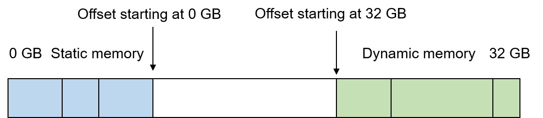
Fig. 6.4.3 Memory allocation using double offsetpointers
6.4.3. Memory Reuse
In a machine learning system, memory reuse is achieved by analyzing the lifespan of a tensor and, once it reaches the end of its lifespan, releasing its device memory back to the memory pool for future reuse by other tensors. The objective of memory reuse is to enhance memory utilization and enable the accommodation of larger models within the constraints of limited device memory. By reusing memory instead of continuously allocating new memory for tensors, the system can optimize memory utilization and mitigate the memory limitations inherent in deep learning computations.
Figure Fig. 6.4.2 provides an example, where output 1 becomes unused once the computation of the BatchNorm operator is complete. In this case, the device memory of output 1 can be reclaimed and reused for output 3 (if output 3 does not require a larger memory size than output 1).
Figure Fig. 6.4.4 depicts memory lifetime using coordinate charts. The horizontal axes represent the tensor lifetime, and the vertical axes represent the memory sizes. During its lifetime, a tensor occupies a specific amount of device memory. The objective of memory allocation is to find an optimal solution that accommodates the maximum number of non-conflicting rectangular blocks (each denoting a tensor’s lifetime and memory size) in the same memory. In Figure Fig. 6.4.4, the memory can accommodate only four rectangular blocks (i.e., tensors T0, T1, T2, and T3) when no memory reuse policy is applied, as shown in the left chart.
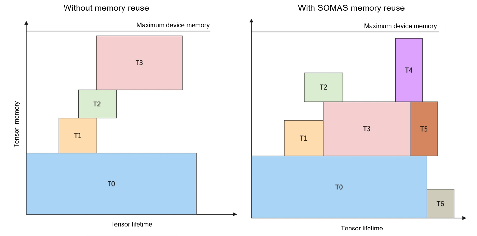
Fig. 6.4.4 Memory lifetimecharts
To determine an appropriate memory reuse policy, we face an NP-complete problem. AI frameworks often employ greedy algorithms, such as best-fit, which allocate memory by searching for the smallest available block in the memory pool one at a time. However, this approach only yields a locally optimal solution rather than a globally optimal one. To approximate a globally optimal solution, a method called Safe Optimized Memory Allocation Solver (SOMAS) can be considered.
SOMAS addresses the computational graph by conducting aggregative analysis on parallel streams and data dependencies. This analysis reveals the ancestor-descendant relationships between operators. By generating a global set of mutually exclusive constraints concerning the lifetime of each tensor, SOMAS combines multiple heuristic algorithms to achieve an optimal solution for static memory planning. Through SOMAS, an optimized memory reuse outcome is obtained, resulting in increased reusable memory.
As shown in the right chart of Figure Fig. 6.4.4, with the SOMAS algorithm, the number of tensors allowed in the same memory is increased to seven.
6.4.4. Optimization Techniques for Memory Allocation
In the following, we describe the typical optimization techniques for memory allocation.
6.4.4.1. Memory Fusion
Commonly used memory allocation methods operate at the tensor level, often resulting in discontinuous device addresses across tensors. However, certain specialized operators, like AllReduce for communication, require contiguous memory allocation. Executing a communication operator involves waiting for communication, which is a significant performance bottleneck in large-scale distributed systems. It includes data transfer and computation. To minimize communication time, we can fuse multiple communication operators into a composite operator. This allows for contiguous memory allocation of the operator input, as depicted in Figure Fig. 6.4.5.
Additionally, the time spent in communication can be reduced during the weight initialization task in distributed neural network training. This task involves broadcasting the initialized weight from one process to all processes. If a network contains multiple weights (which is often the case), these broadcasts are repeated. To minimize communication time in this scenario, a typical approach is to allocate contiguous memory addresses to all weights on the network and then perform a single broadcast operation.
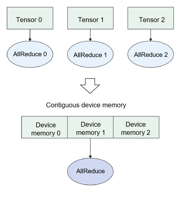
Fig. 6.4.5 Memory fusion of communicationoperators
6.4.4.2. In-place Operators
In the memory allocation process depicted in
Figure :numref:ch07/ch07-compiler-backend-memory-02, the input and
output of each operator are assigned different memory addresses.
However, this approach can lead to memory waste and performance
degradation for several other operators. Examples include optimizer
operators used to update neural network weights, Python’s += or
*= operators that modify variable values, and the a[0]=b
operator that updates the value of a[0] with b. These operators
share a common purpose: updating the input value. The concept of
in-place can be illustrated using the a[0]=b operator.
In the original implementation shown on the left of Figure
Fig. 6.4.6, the operator involves
three steps: copying tensor a to tensor a’, assigning tensor
b to tensor a’, and then copying tensor a’ back to tensor
a. However, by performing the operation in-place, as depicted on the
right of Figure Fig. 6.4.6, this
process is simplified to a single step: copying tensor b to the
position corresponding to tensor a. This reduces data copy time by
eliminating two copies and eliminates the need to allocate memory for
tensor a’.
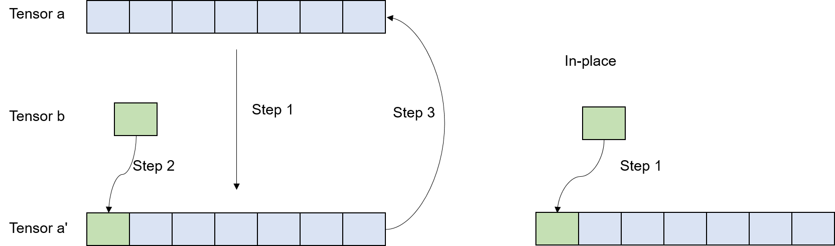
Fig. 6.4.6 Memory allocation of an in-placeoperator
6.4.5. Data Compression
Deep neural networks (DNNs) in modern training heavily rely on GPUs to effectively train intricate networks with hundreds of layers. A prominent challenge faced by both researchers and industry professionals is the constraint imposed by the available GPU main memory as networks become deeper. This limitation restricts the size of networks that can be trained. To address this issue, researchers have recognized the value of employing DNN-layer-specific encoding schemes. Consequently, they have directed their attention towards storing encoded representations of the intermediate layer outputs (feature maps) that are required for the backward pass. These encoded representations are stored during the temporal gap between their uses and are decoded only when needed for the backward pass. The full-fidelity feature maps are promptly discarded after use, resulting in a noteworthy reduction in memory consumption.
6.4.6. Memory Swap
Machine learning frameworks frequently necessitate users to optimize their memory utilization to guarantee that the DNN can be accommodated within the memory capacity of the GPU. This constraint restricts researchers from thoroughly investigating diverse machine learning algorithms, compelling them to make concessions either in terms of network architecture or by distributing the computational load across multiple GPUs. One feasible approach is to incorporate DRAM to facilitate memory swapping. By transferring temporarily inactive data to DRAM, we can optimize GPU utilization. In recent studies, researchers have implemented a cautious approach to allocating GPU memory for the immediate computational needs of a specific layer. This strategy effectively reduces both the maximum and average memory usage, enabling researchers to train more extensive networks. To elaborate further, the researchers promptly release feature maps from GPU memory in the absence of any potential reuse. Alternatively, if there is a possibility of future reuse but no immediate requirement, the feature maps are offloaded to CPU memory and subsequently prefetched back to GPU memory.
The fundamental concept behind memory swapping is straightforward and inherent. However, its implementation remains challenging and necessitates prior expertise in our compiler frontend. One such expertise involves maximizing the overlap between computation and data swapping time. A precise cost model is essential for evaluating the estimated time required for data movement and the time cost associated with each layer in DNN (Deep Neural Network). Additionally, there are numerous strategies to explore in auto scheduling and auto tuning. Fortunately, there is an abundance of literature available that addresses these issues. For additional information, please refer to the Further Readings section.