8.4. Architecture of Machine Learning Clusters
Distributed model training is usually implemented in a compute cluster. Next, we will introduce the composition of a compute cluster and explore the design of a cluster network.
Figure Fig. 8.4.1 shows the typical architecture of a machine learning cluster. There are many servers deployed in such a cluster, and each server has several hardware accelerators. To facilitate server management, multiple servers are placed into one rack, which is connected to a top of rack (ToR) switch. If ToR switches are fully loaded but more new racks need to be connected, we can add a spine switch between ToR switches. Such a structure forms a multi-level tree. It is worth noting that cross-rack communication within a cluster may encounter network bottlenecks. This is because the network links used to construct the cluster network have the same specifications (necessary to facilitate hardware procurement and device management), increasing the probability of network bandwidth oversubscription on the network links from the ToR switches to the spine switch.
Network bandwidth oversubscription can be defined as a situation wherein the peak bandwidth required exceeds the actual bandwidth available on the network. In the cluster shown in Figure Fig. 8.4.1, when server 1 and server 2 send data to server 3 through their respective network links (say 10 Gb/s of data), ToR switch 1 aggregates the data (that is, 20 Gb/s) and sends it to spine switch 1. However, because there is only one network link (10 Gb/s) between spine switch 1 and ToR switch 1, the peak bandwidth required is twice the actual bandwidth available, hence network bandwidth oversubscription. In real-world machine learning clusters, the ratio between peak bandwidth and actual bandwidth is generally between 1:4 and 1:16. One approach for avoiding network bottlenecks is to restrict network communication within individual racks. This approach has become a core design requirement for distributed machine learning systems.
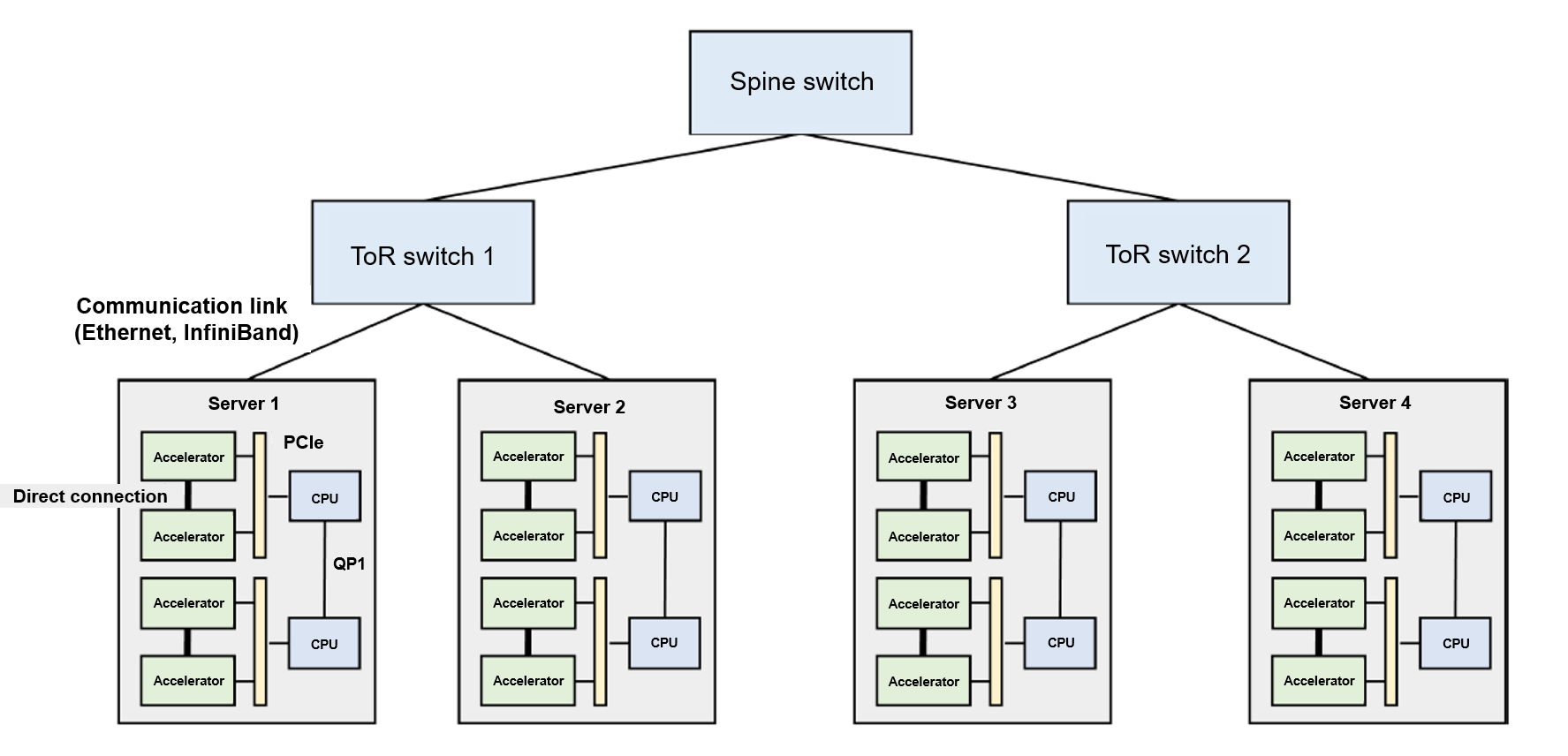
Fig. 8.4.1 Architecture of a machine learningcluster
So, how much network bandwidth is required for training a large-scale neural network in a compute cluster? Assume a neural network has hundreds of billions of parameters (e.g., GPT-3 — a huge language model released by OpenAI — has nearly 175 billion parameters). If each parameter is expressed with a 32-bit floating-point number, a single model replica in data parallelism mode will generate 700 GB (175 billion \(*\) 4 bytes) of local gradient data in each round of training iteration. If there are three model replicas, at least 1.4 TB [700 GB \(*\) \((3-1)\)] of gradient data needs to be transmitted. This is because for \(N\) replicas, only \(N-1\) of them need to be transmitted for computation. To ensure that the model replicas will not diverge from the parameters in the main model, the average gradient — once computed — is broadcast to all model replicas (1.4 TB of data) for updating local parameters in these model replicas.
Currently, machine learning clusters generally use Ethernet to construct networks between different racks. The bandwidth of mainstream commercial Ethernet links ranges from 10 Gb/s to 25 Gb/s. 1 Using Ethernet to transmit massive gradients will encounter severe transmission latency. Because of this, new machine learning clusters (such as NVIDIA DGX) are often configured with the faster InfiniBand. A single InfiniBand link can provide 100 Gb/s or 200 Gb/s bandwidth. Even this high-speed network still faces high latency when transmitting TB-level local gradients. Even if network latency is ignored, it takes at least 40 seconds to transmit 1 TB of data on a 200 Gb/s link.
To address this issue, InfiniBand uses remote direct memory access (RDMA) as the core of its programming interfaces. RDMA enables InfiniBand to provide high-bandwidth, low-latency data read and write functions. As such, its programming interfaces are vastly different from the TCP/IP socket interfaces used by conventional Ethernet. For compatibility purposes, people use the IP-over-InfiniBand (IPoIB) technology, which ensures that legacy applications can invoke socket interfaces whereas the underlying layer invokes the RDMA interfaces of InfiniBand through IPoIB.
To support multiple accelerators (typically 2–16) within a server, a common practice is to build a heterogeneous network on the server. Take server 1 in Figure Fig. 8.4.1 as an example. This server is equipped with two CPUs, which communicate with each other through QuickPath Interconnect (QPI). Within a CPU interface (socket), the accelerator and CPU are connected by a PCIe bus. Accelerators use high-bandwidth memory (HBM), which offers much more bandwidth than PCIe does. A prominent example is the NVIDIA A100 server: In this server, HBM offers 1935 GB/s bandwidth, whereas PCIe 4.0 offers only 64 GB/s bandwidth. PCIe needs to be shared by all accelerators within the server, meaning that it becomes a significant communication bottleneck when multiple accelerators simultaneously transmit data through PCIe. To solve this problem, machine learning servers tend to use accelerator high-speed interconnect technologies (e.g., NVIDIA GPU NVLink). Such technology bypasses PCIe to achieve high-speed communication. A prominent example is NVIDIA A100 GPU — its NVLink provides 600 GB/s bandwidth, enabling accelerators to transmit large amounts of data to each other.