6.5. Operator Compiler

Operator compilers are used for compiling and optimizing operators, which may be part of a neural network or come from the code implemented in a domain-specific language (DSL). The compilation is the process of transforming the source code from one representation into another.

The objective of an operator compiler is to improve the execution performance of operators. An operator compiler accepts tensor computation logic described in dynamic languages (e.g., Python) as the input and outputs executable files on specific AI processors.

6.5.1. Scheduling Strategy

An operator compiler abstracts the execution of statements in an operator implementation into “scheduling strategies”. Since an operator typically consists of multiple statements, the focus lies in determining the scheduling strategy for the statements within the operator. This strategy encompasses considerations such as the calculation order, data block movement, and other relevant factors.

If ignoring the specific processor architecture, for the best performance, we only need to load all input tensors to the computation core based on the computational logic of the operator and access the result from the core for storage. Computational logic refers to basic arithmetic operations (e.g., addition, subtraction, multiplication, and division) and other function expressions (e.g., convolution, transposition, and loss functions).

Modern computer memory hierarchy looks like a pyramid structure, as shown in Figure Fig. 6.5.1. As we move up the pyramid, the storage elements have a higher cost but a faster access time.

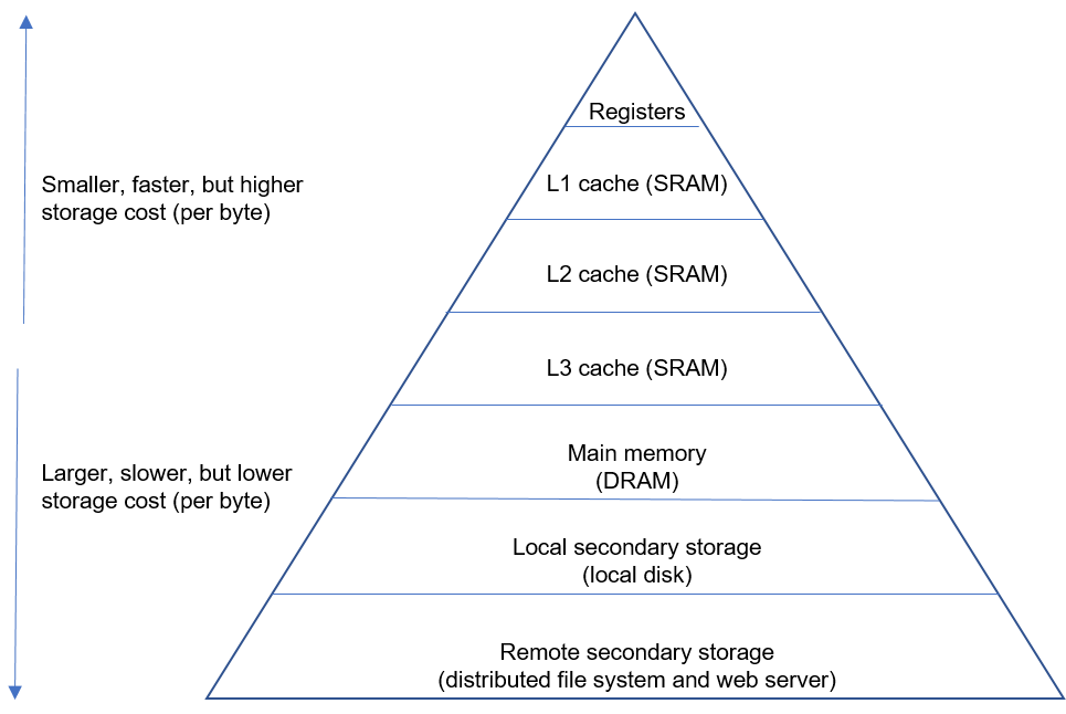
Fig. 6.5.1 Modern computer memoryhierarchy

Such hardware design leads to two basic types of locality:

(1) Temporal locality: the tendency to access the same memory location several times in quick succession. As such, accessing the same location in the L1 cache several times is more efficient than accessing different locations in the L1 cache several times.

(2) Spatial locality: the tendency to access nearby memory locations in quick succession. As such, accessing nearby locations in the L1 cache several times is more efficient than moving back and forth between the L1 cache and the main memory.

Both types of locality help improve system performance. Specifically, in order to improve the data access speed, data to be repeatedly processed can be placed in fixed nearby memory locations when possible.

For a serial computational task, it is also possible to decouple the data part from the logic part and generate a range of independent groups of data that can be executed in parallel, as shown in Figure Fig. 6.5.2.

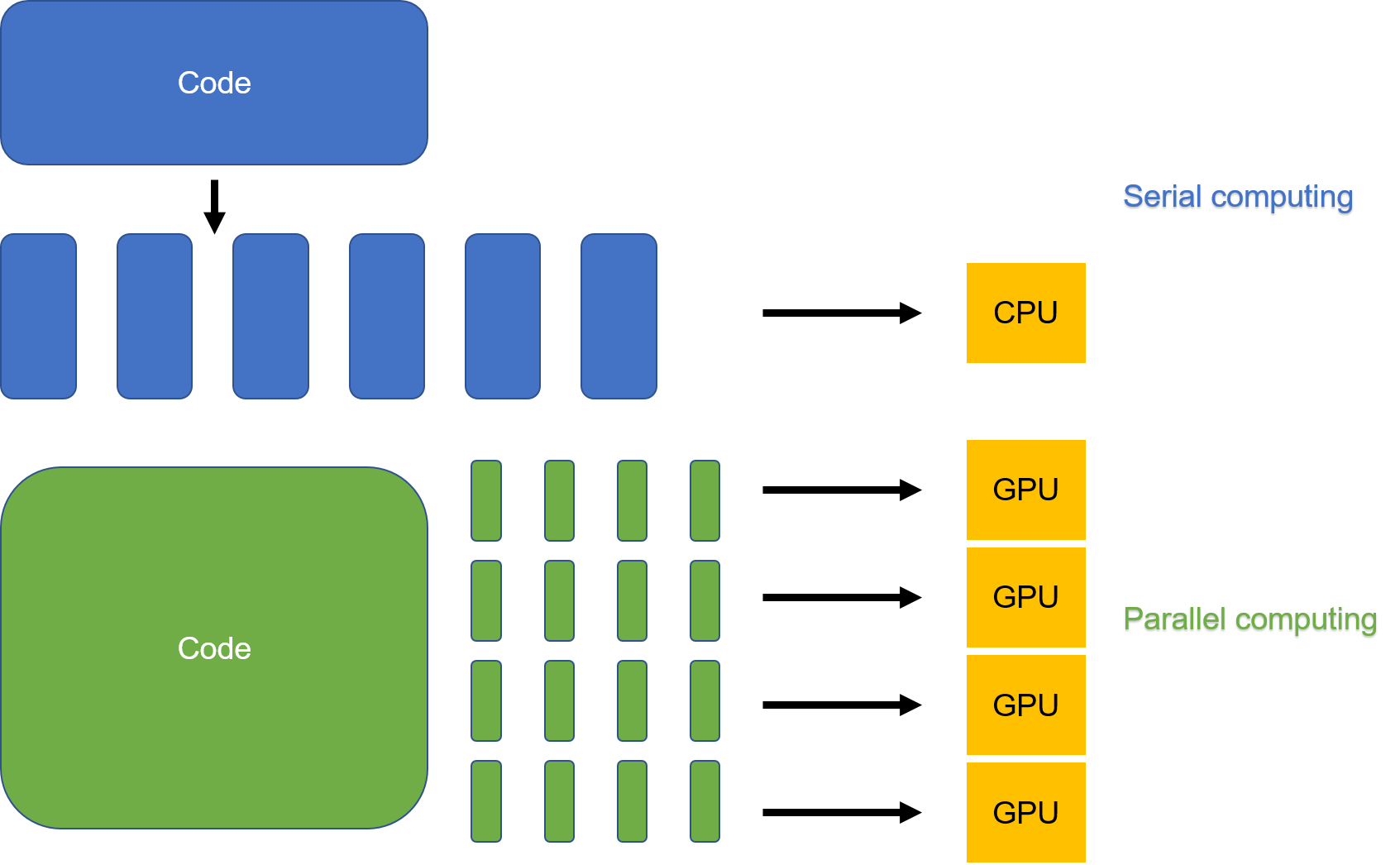
Fig. 6.5.2 Serial computing and parallelcomputing

These specific data-oriented operations performed at program runtime are referred to as schedules. A schedule defines the following aspects:

1. When and where should each value in a function be calculated?

2. Where is data stored?

(3) How long does it take to access each value between those calculated using preorder structure consumers? And when is independent recomputation performed by each such value?

Simply put, a scheduling strategy is defined by a set of algorithms designed during compilation based on the characteristics of target hardware architecture to improve locality and parallelism. The purpose of this is to ensure that the resulting executable file delivers optimal performance at runtime. These algorithms have no effect on the computation result; instead, they only adjust the computation process in order to shorten the computation time.

6.5.2. Combining Scheduling Strategies

In the realm of operator compilers, a common optimization technique involves combining multiple abstracted scheduling strategies into a comprehensive and efficient scheduling set through manual template matching. However, this approach may not be fine-tuned and can be labor-intensive when applied to achieve refined optimization across different operators. To illustrate this, let’s consider an optimization algorithm implemented in the Tensor Virtual Machine (TVM). It accelerates and optimizes a multiply-accumulate code segment on the CPU by combining several fundamental scheduling strategies.

In Code lst:before_tvm, the basic computational logic is as follows: Initialize tensor C, multiply tensor A by tensor B, and accumulate the results to tensor C.

lst:before_tvm

for (m: int32, 0, 1024) {
  for (n: int32, 0, 1024) {
    C[((m*1024) + n)] = 0f32
      for (k: int32, 0, 1024) {
        let cse_var_2: int32 = (m*1024)
          let cse_var_1: int32 = (cse_var_2 + n)
            C[cse_var_1] = (C[cse_var_1] + (A[(cse_var_2 + k)]*B[((k*1024) + n)]))
      }
  }
}

Assuming that the data type is float and that tensors A, B, and C are of size 1024 \(\times\) 1024, then the total memory required by the tensors is 1024 \(\times\) 1024 \(\times\) 3 \(\times\) sizeof(float) = 12 MB. This far exceeds the capacity of common caches (e.g., the L1 cache is 32 KB). Therefore, if we want to compute on Tensor A, B, and C in a single operation, we must store them in the main memory. However, the main memory is distant from the compute core, resulting in significantly lower access efficiency compared to using the cache for storage.

There are several scheduling strategies that can help improve performance: tile, reorder, and split. The size of the L1 cache is 32 KB. To ensure that data used in every computation step is stored in the cache, tiling based on the factors of 32 is performed. In this way, only the tiny block formed by m.inner\(\times\)n.inner needs to be taken into account, and memory access of the innermost tiny block is independent of the outer loops. A tiny block will occupy only 32 \(\times\) 32 \(\times\) 3 \(\times\) sizeof(float), which is 12 KB in the cache. The optimized code is shown in Code lst:after_tvm. We perform tiling on loops m and n based on factor 32 as the previous analysis. Similarly, we tile the loop k based on factor 4, then reorder the k.outer and k.inner axis as the outermost axis.

lst:after_tvm

// Obtain an outer loop by tiling for (m: int32, 0, 1024) based on factor 32.
for (m.outer: int32, 0, 32) {
  // Obtain an outer loop by tiling for (n: int32, 0, 1024) based on factor 32.
  for (n.outer:
    // Obtain an inner loop by tiling for (m: int32, 0, 1024) based on factor 32.
    for (m.inner.init: int32, 0, 32) {
      // Obtain an inner loop by tiling for (n: int32, 0, 1024) based on factor 32.
      for (n.inner.init: int32, 0, 32) {
        // Obtain the corresponding factors.
        C[((((m.outer*32768) + (m.inner.init*1024)) + (n.outer*32)) + n.inner.init)] = 0f32
      }
    }
    // Obtain an outer loop by splitting for (k: int32, 0, 1024) based on factor 4, with reorder.
    for (k.outer: int32, 0, 256) {
      // Obtain an outer loop by splitting for (k: int32, 0, 1024) based on factor 4, with reorder.
      for (k.inner: int32, 0, 4) {
        // Obtain an inner loop by tiling for (m: int32, 0, 1024) based on factor 32.
        for (m.inner: int32, 0, 32) {
          // Obtain an inner loop by tiling for (n: int32, 0, 1024) based on factor 32.
          for (n.inner: int32, 0, 32) {
            // Outer axis factor obtained by tiling along axis n
            let cse_var_3: int32 = (n.outer*32)
            // Outer axis & inner axis factors obtained by tiling along axis m
            let cse_var_2: int32 = ((m.outer*32768) + (m.inner*1024))
            // Outer axis & inner axis factors obtained by tiling along axes m & n
            let cse_var_1: int32 = ((cse_var_2 + cse_var_3) + n.inner)
            // Split the computational logic into different layers so that data involved every loop can be stored in the cache.
            C[cse_var_1] = (C[cse_var_1] + (A[((cse_var_2 + (k.outer*4)) + n.inner)] * B[((((k.outer*4096) + (k.inner*1024)) + cse_var_3) + n.inner)]))
          }
        }
      }
    }
  }
}

6.5.3. Finding Optimized Strategies with Polyhedral Models

Another optimization approach is to automatically select an operator schedule from a schedule search space. A good example of this idea is the polyhedral compilation. They improve the generalization of operator compilation at the expense of prolonged compile time.

Polyhedral compilation mainly optimizes the loops in user code by abstracting each loop into a multidimensional space, computing instances into points in the space, and dependencies between the instances into lines in the space. The main idea of this algorithm is to model the memory access characteristics in code and adjust the execution order of each instance within each loop. In this way, it aims to enable better locality and parallelism of the loop code under the new schedule.

Code lst:before_poly is used as an example to describe the algorithm.

lst:before_poly

for (int i = 0; i < N; i++)
  for (int j = 1; j < N; j++)
    a[i+1][j] = a[i][j+1] - a[i][j] + a[i][j-1];

As shown in Figure Fig. 6.5.3, a memory access structure is first modeled by using the polyhedral model algorithm, and then dependencies (denoted by arrows) between instances (denoted by nodes) are analyzed.

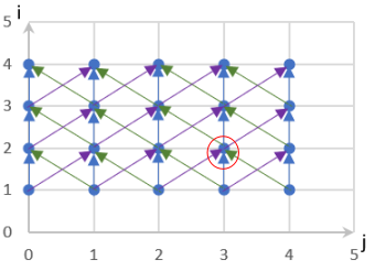
Fig. 6.5.3 Polyhedral model of the samplecode

Complex dependency analysis and schedule transformation are then performed to obtain an optimal solution that fits the memory model. Using the polyhedral model algorithm, the code is optimized to that shown in Code lst:after_poly.

lst:after_poly

for (int i_new = 0; i_new < N; i_new++)
  for (int j_new = i+1; j_new < i+N; j_new++)
    a[i_new+1][j_new-i_new] = a[i_new][j_new-i_new+1] - a[i_new][j_new-i_new] + a[i_new][j_new-i_new-1];

The resulting code looks relatively complex. We can model the code (as shown in Figure Fig. 6.5.4) to determine its performance improvements. Through dependency analysis, we find that the loop dependencies present in the source code are removed in the optimized code, thereby increasing the opportunities for parallel computing. Specifically, parallel computing is possible when the loop dependencies are partitioned along the dashed lines based on the green blocks, as shown in Figure Fig. 6.5.4.

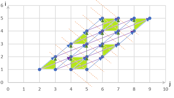
Fig. 6.5.4 Optimization result with the polyhedralmodel

We have only introduced the Polyhedral Compilation technique in this section. However, there are other optimization techniques available, such as Ansor, which is a heuristic searching method with pruning.

6.5.4. Adaptation to Instruction Sets

We have previously explored the optimization techniques of operator compilers. In this section, we build on this foundation to examine how operator compilers adapt to instruction sets on different chips. Typically, a general-purpose compiler is designed to be compatible with as many backend architectures and instruction sets as possible. However, this can present challenges when the compiler must handle backends with different architectures and instruction sets.

Two common programming models adopted by AI processors are single instruction, multiple data (SIMD) and single instruction, multiple threads (SIMT). As shown in Figures Fig. 6.5.5 and Fig. 6.5.6, respectively, SIMD corresponds to chips with vector instructions, while SIMT corresponds to chips that support multiple threads. Recently, some chips have begun to combine both programming models in order to support both multithreaded parallel computing and vector instructions. When handling different programming models, an operator compiler adopts different optimization strategies, such as vectorization.

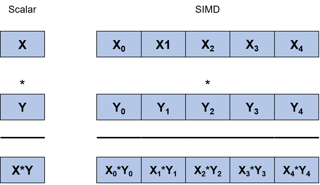
Fig. 6.5.5 SIMD diagram

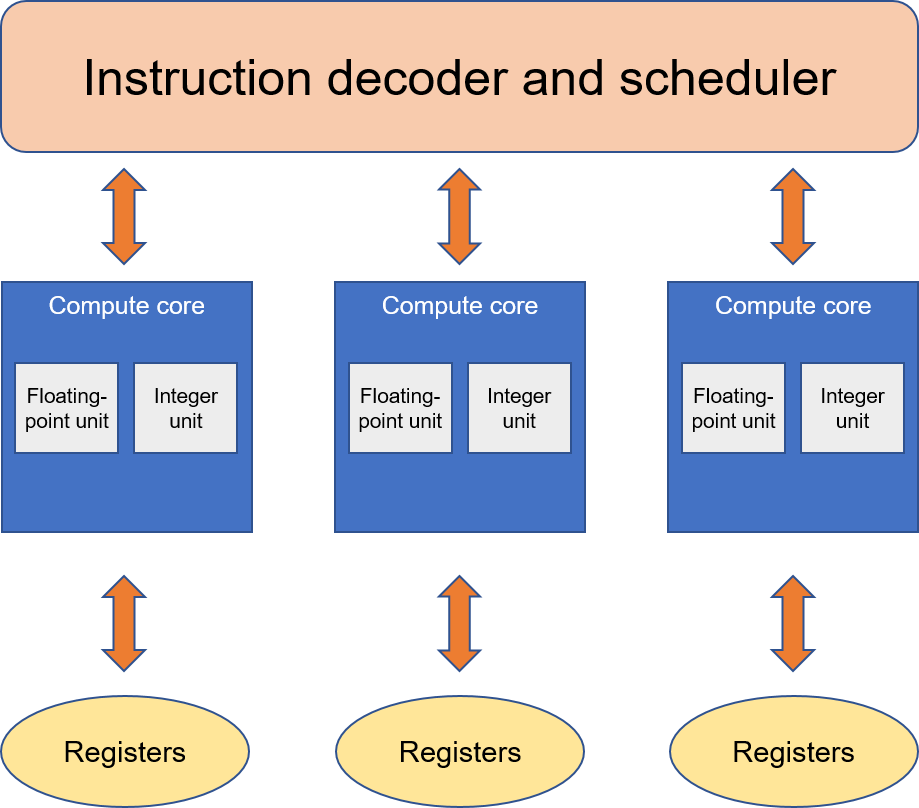
Fig. 6.5.6 SIMT diagram

Operator compilers place a strong emphasis on differentiated support in the frontend, midend, and backend. In the frontend, support for multiple backend instruction sets is added, allowing AI programmers to focus on algorithm logic without having to worry about chip differences. In the midend, the architectures of different chips are identified, which allows for specific optimization methods to be implemented for each chip. When generating backend code, the instruction sets of different chips are further identified to ensure efficient execution on target chips.

6.5.5. Expression Ability

The representation capability of an operator compiler is important because it determines how well the frontend can express the input code in an IR without loss of syntax information. The frontend of an operator compiler is often fed with code programmed in flexible languages (e.g., PyTorch code written in Python). However, flexible expressions (e.g., indexing and view syntax in Python) pose high requirements on the frontend expression ability of operator compilers. From the model perspective, managing the inputs of an operatorn often contain many control flow statements. Also, some models allow for dynamic-shape operators whose shapes vary with control flow decisions across iterations.

Additionally, there are a large number of operators that may not have optimized implementation provided by the accelerator libraries (e.g., cuDNN) directly. This phenomenon is referred to as long tail operators. However, the long tail operators can have highly flexible syntax or abundant control flow statements and sometimes support dynamic shapes, making it extremely difficult for the frontend of existing operator compilers to express, optimize, or accelerate them. Consequently, such operators have to be executed by the Python interpreter or slow virtual machines, leading to a performance bottleneck in network execution. This is why it is imperative to improve the expression ability of the operator compiler frontend.