9.5. Model Inference

After conversion and compression, a trained model needs to be deployed on the computation hardware in order to execute inference. Such execution involves the following steps:

1. Preprocessing: Process raw data to suit the network input.

2. Inference execution: Deploy the model resulting from offline conversion on the device to execute inference and compute the output based on the input.

3. Postprocessing: Further process the output of the model, for example, by threshold filtering.

9.5.1. Preprocessing and Postprocessing

1. Preprocessing

Raw data, such as images, voices, and texts, is so disordered that machine learning models cannot identify or extract useful information from it. Preprocessing is intended to convert such into tensors that work for machine learning networks, eliminate irrelevant information, restore useful true information, enhance the detectability of relevant information, and simplify the data as much as possible. In this way, reliability indicators related to feature extraction, image segmentation, matching, and recognition of the models can be improved.

The following techniques are often used in data preprocessing:

1. Feature encoding: Encode the raw data that describes features into numbers and input them to machine learning models which can process only numerical values. Common encoding approaches include discretization, ordinal encoding, one-hot encoding, and binary encoding.

2. Normalization: Modify features to be on the same scale without changing the correlation between them, eliminating the impact of dimensions between data indicators. Common approaches include Min-Max normalization that normalizes the data range, and Z-score normalization that normalizes data distribution.

3. Outliner processing: An outlier is a data point that is distant from all others in distribution. Elimination of outliers can improve the accuracy of a model.

2. Postprocessing

After model inference, the output data is transferred to users for postprocessing. Common postprocessing techniques include:

1. Discretization of contiguous data: Assume we expect to predict discrete data, such as the quantity of a good, using a model, but a regression model only provides contiguous prediction values, which have to be rounded or bounded.

2. Data visualization: This technique uses graphics and tables to represent data so that we can find relationships in the data in order to support analysis strategy selection.

3. Prediction range widening: Most values predicted by a regression model are concentrated in the center, and few are in the tails. For example, abnormal values of hospital laboratory data are used to diagnose diseases. To increase the accuracy of prediction, we can enlarge the values in both tails by widening the prediction range and multiplying the values that deviate from the normal range by a coefficient to

9.5.2. Parallel Computing

Most inference models have a multi-thread mechanism that leverages the capabilities of multiple cores in order to achieve performance improvements. In this mechanism, the input data of operators is partitioned, and multiple threads are used to process different data partitions. This allows operators to be computed in parallel, thereby multiplying the operator performance.

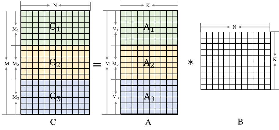
Fig. 9.5.1 Data partitioning for matrixmultiplication

In Figure Fig. 9.5.1, the matrix in the multiplication can be partitioned according to the rows of matrix A. Three threads can then be used to compute A1 * B, A2 * B, and A3 * B (one thread per computation), implementing multi-thread parallel execution of the matrix multiplication.

To facilitate parallel computing of operators and avoid the overhead of frequent thread creation and destruction, inference frameworks usually have a thread pooling mechanism. There are two common practices:

1. Open Multi-Processing (OpenMP) API: OpenMP is an API that supports concurrency through memory sharing across multiple platforms. It provides interfaces that are commonly used to implement operator parallelism. An example of such an interface is parallel for, which allows for loops to be concurrently executed by multiple threads.

2. Framework-provided thread pools: Such pools are more lightweight and targeted at the AI domain compared with OpenMP interfaces, and can deliver better performance.

9.5.3. Operator Optimization

When deploying an AI model, we want model training and inference to be performed as fast as possible in order to obtain better performance. For a deep learning network, the scheduling of the framework takes a short period of time, whereas operator execution is often a bottleneck for performance. This section introduces how to optimize operators from the perspectives of hardware instructions and algorithms.

1. Hardware instruction optimization

Given that most devices have CPUs, the time that CPUs spend processing operators has a direct impact on the performance. Here we look at the methods for optimizing hardware instructions on ARM CPUs.

1) Assembly language

High-level programming languages such as C++ and Java are compiled as machine instruction code sequences by compilers, which often have a direct influence on which capabilities these languages offer. Assembly languages are close to machine code and can implement any instruction code sequence in one-to-one mode. Programs written in assembly languages occupy less memory, and are faster and more efficient than those written in high-level languages.

In order to exploit the advantages of both types of languages, we can write the parts of a program that require better performance in assembly languages and the other parts in high-level languages. Because convolution and matrix multiplication operators in deep learning involve a large amount of computation, using assembly languages for code necessary to perform such computation can improve model training and inference performance by dozens or even hundreds of times.

Next, we use ARMv8 CPUs to illustrate the optimization related to hardware instructions.

2) Registers and NEON instructions

Each ARMv8 CPU has 32 NEON registers, that is, v0 to v31. As shown in Figure Fig. 9.5.2, NEON register v0 can store 128 bits, which is equal to the capacity of 4 float32, 8 float16, or 16 int8.

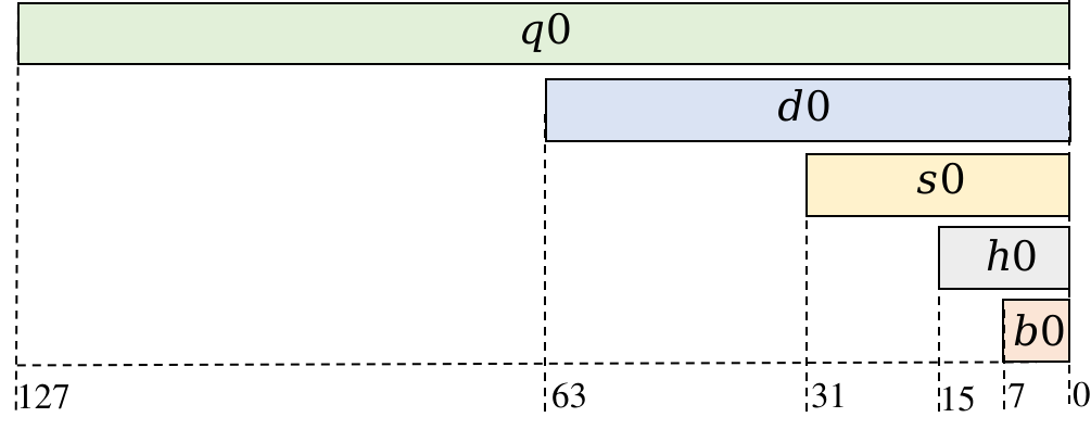
Fig. 9.5.2 Structure of the NEON register v0 of an ARMv8CPU

The single instruction multiple data (SIMD) method can be used to improve the data access and computing speed on this CPU. Compared with single data single instruction (SISD), the NEON instruction can process multiple data values in the NEON register at a time. For example, the fmla instruction for floating-point data is used as fmla v0.4s, v1.4s, v2.4s. As depicted in Figure Fig. 9.5.3, the products of the corresponding floating-point values in registers v1 and v2 are added to the value in v0.

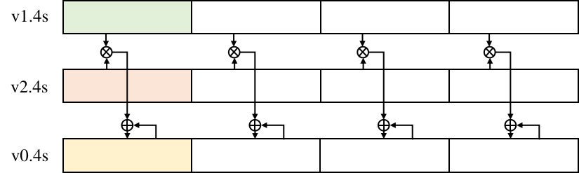
Fig. 9.5.3 fmla instructioncomputing

3) Assembly language optimization

For assembly language programs with known functions, computational instructions are usually fixed. In this case, non-computational instructions are the source the performance bottleneck. The structure of computer storage devices resembles a pyramid, as shown in Figure Fig. 9.2.1. The top layer has the fastest speed but the smallest space; conversely, the bottom layer has the largest space but the slowest speed. L1 to L3 are referred to as caches. When accessing data, the CPU first attempts to access the data from one of its caches. If the data is not found, the CPU then accesses an external main memory. Cache hit rate is introduced to measure the proportion of data that is accessed from the cache. In this sense, the cache hit rate must be maximized to improve the program performance.

There are some techniques to improve the cache hit rate and optimize the assembly performance:

1. Loop unrolling: Use as many registers as possible to achieve better performance at the cost of increasing the code size.

2. Instruction reordering: Reorder the instructions of different execution units to improve the pipeline utilization, thereby allowing instructions that incur latency to be executed first. In addition to reducing the latency, this method also reduces data dependency before and after the instruction.

3. Register blocking: Block NEON registers appropriately to reduce the number of idle registers and reuse more registers.

4. Data rearrangement: Rearrange the computational data to ensure contiguous memory reads and writes and improve the cache hit rate.

5. Instruction prefetching: Load the required data from the main memory to the cache in advance to reduce the access latency.

2. Algorithm optimization

For most AI models, 90% or more of the inference time of the entire network is spent on computing convolution and matrix multiplication operators. This section focuses on the optimization of convolution operator algorithms, which can be applied to various hardware devices. The computation of convolution can be converted into the multiplication of two matrices, and we have elaborated on the optimization of the GEMM algorithm in Section Parallel Computing. For different hardware, appropriate matrix blocking can optimize data load/store efficiency and instruction parallelism. This helps to maximize the utilization of the hardware’s computing power, thereby improving the inference performance.

(1) Img2col

Img2col is often used to convert convolution into matrix multiplication. Convolutional layers typically operate on 4D inputs in NHWC format. Figure Fig. 9.5.4 is a diagram of convolution. The input shape is (1, IH, IW, IC), the convolution kernel shape is (OC, KH, KW, IC), and the output shape is (1, OH, OW, OC).

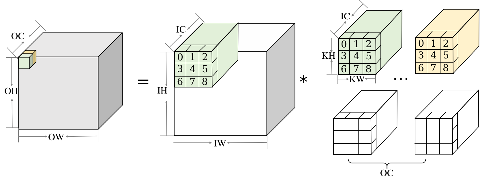
Fig. 9.5.4 Generalconvolution

As shown in Figure Fig. 9.5.5, the Img2col rules for convolution are as follows: The input is reordered to obtain the matrix on the right. The number of rows corresponds to the number of OH * OW outputs. For a row vector, Img2col processes KH * KW data points of each input channel in sequence, from the first channel to channel IC.

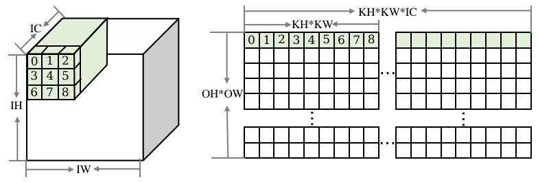
Fig. 9.5.5 Img2col on the convolutioninput

As shown in Figure Fig. 9.5.6, the weights are rearranged. One convolution kernel is expanded into one column of the weight matrix. This means that there are OC columns in total. On each column vector, KH * KW data values on the first input channel are arranged first, and then on subsequent channels until the channel IC. In this manner, the convolution operation is converted into the multiplication of two matrices. In practice, the data rearrangement of Img2col and GEMM is performed simultaneously to save time.

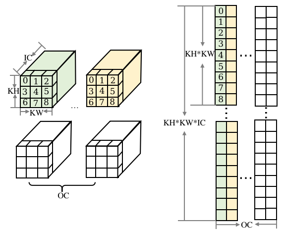
Fig. 9.5.6 Img2col on the convolutionkernel

(2) Winograd

Convolution is essentially considered as matrix multiplication. The time complexity of multiplying two 2D matrices is \(O(n^3)\). The Winograd algorithm can reduce the complexity of matrix multiplication.

Assume that a 1D convolution operation is denoted as F(\(m\), \(r\)), where \(m\) indicates the number of outputs, and \(r\) indicates the number of convolution kernels. The input is \(\textit{\textbf{d}}=[d_0 \ d_1 \ d_2 \ d_3]\), and the convolution kernel is \(g=[g_0 \ g_1 \ g_2]^{\rm T}\). The convolution operation may be written using matrices as Equation ch-deploy/conv-matmul-one-dimension, which contains six multiplications and four additions.

(9.5.1)\[\begin{split}\textit{\textbf{F}}(2, 3)= \left[ \begin{matrix} d_0 & d_1 & d_2 \\ d_1 & d_2 & d_3 \end{matrix} \right] \times \left[ \begin{matrix} g_0 \\ g_1 \\ g_2 \end{matrix} \right]= \left[ \begin{matrix} y_0 \\ y_1 \end{matrix} \right]\end{split}\]

:eqlabel:equ:ch-deploy/conv-matmul-one-dimension

In the preceding equation, there are repeated elements \(d_1\) and \(d_2\) in the input matrix. As such, there is space for optimization for matrix multiplication converted from convolution compared with general matrix multiplication. The matrix multiplication result may be obtained by computing an intermediate variable \(m_0-m_3\), as shown in Equation ch-deploy/conv-2-winograd:

(9.5.2)\[\begin{split}\textit{\textbf{F}}(2, 3)= \left[ \begin{matrix} d_0 & d_1 & d_2 \\ d_1 & d_2 & d_3 \end{matrix} \right] \times \left[ \begin{matrix} g_0 \\ g_1 \\ g_2 \end{matrix} \right]= \left[ \begin{matrix} m_0+m_1+m_2 \\ m_1-m_2+m_3 \end{matrix} \right]\end{split}\]

:eqlabel:equ:ch-deploy/conv-2-winograd

where \(m_0-m_3\) are computed as Equation ch-deploy/winograd-param:

(9.5.3)\[\begin{split}\begin{aligned} m_0=(d_0-d_2) \times g_0 \\ m_1=(d_1+d_2) \times (\frac{g_0+g_1+g_2}{2}) \\ m_2=(d_0-d_2) \times (\frac{g_0-g_1+g_2}{2}) \\ m_3=(d_1-d_3) \times g_2 \end{aligned}\end{split}\]

:eqlabel:equ:ch-deploy/winograd-param

The indirect computation of r1 and r2 by computing \(m_0-m_3\) involves four additions of the input \(d\) and four multiplications and four additions of the output \(m\). Because the weights are constant during inference, the operations on the convolution kernel can be performed during graph compilation, which is excluded from the online runtime. In total, there are four multiplications and eight additions — fewer multiplications and more additions compared with direct computation (which has six multiplications and four additions). In computer systems, multiplications are generally more time-consuming than additions. Decreasing the number of multiplications while adding a small number of additions can accelerate computation.

In a matrix form, the computation can be written as Equation ch-deploy/winograd-matrix, where \(\odot\) indicates the multiplication of corresponding locations, and A, B, and G are all constant matrices. The matrix here is used to facilitate clarity — in real-world use, faster computation can be achieved if the matrix computation is performed based on the handwritten form, as provided in Equation ch-deploy/winograd-param.

(9.5.4)\[\textit{\textbf{Y}}=\textit{\textbf{A}}^{\rm T}(\textit{\textbf{G}}g) \odot (\textit{\textbf{B}}^{\rm T}d)\]

:eqlabel:equ:ch-deploy/winograd-matrix

(9.5.5)\[\begin{split}\textit{\textbf{B}}^{\rm T}= \left[ \begin{matrix} 1 & 0 & -1 & 0 \\ 0 & 1 & 1 & 0 \\ 0 & -1 & 1 & 0 \\ 0 & 1 & 0 & -1 \end{matrix} \right]\end{split}\]

:eqlabel:equ:ch-deploy/winograd-matrix-bt

(9.5.6)\[\begin{split}\textit{\textbf{G}}= \left[ \begin{matrix} 1 & 0 & 0 \\ 0.5 & 0.5 & 0.5 \\ 0.5 & -0.5 & 0.5 \\ 0 & 0 & 1 \end{matrix} \right]\end{split}\]

:eqlabel:equ:ch-deploy/winograd-matrix-g

(9.5.7)\[\begin{split}\textit{\textbf{A}}^{\rm T}= \left[ \begin{matrix} 1 & 1 & -1 & 0 \\ 0 & 1 & -1 & -1 \end{matrix} \right] \\\end{split}\]

:eqlabel:equ:ch-deploy/winograd-matrix-at

In deep learning, 2D convolution is typically used. When F(2, 3) is extended to F(2:math:times2, 3\(\times\)3), it can be written in a matrix form, as shown in Equation ch-deploy/winograd-two-dimension-matrix. In this case, Winograd has 16 multiplications, reducing the computation complexity by 2.25 times compared with 36 multiplications of the original convolution.

(9.5.8)\[\textit{\textbf{Y}}=\textit{\textbf{A}}^{\rm T}(\textit{\textbf{G}}g\textit{\textbf{G}}^{\rm T}) \odot (\textit{\textbf{B}}^{\rm T}d\textit{\textbf{B}})\textit{\textbf{A}}\]

:eqlabel:equ:ch-deploy/winograd-two-dimension-matrix

The logical process of Winograd can be divided into four steps, as shown in Figure Fig. 9.5.7.

Fig. 9.5.7 Winogradsteps

To use Winograd of F(2:math:times2, 3\(\times\)3) for any output size, we need to divide the output into 2\(\times\)2 blocks. We can then perform the preceding four steps using the corresponding input to obtain the corresponding output. Winograd is not limited to solving F(2:math:times2, 3\(\times\)3). For any F(\(m \times m\), \(r \times r\)), appropriate constant matrices A, B, and G can be found to reduce the number of multiplications through indirect computation. However, as \(m\) and \(r\) increase, the number of additions involved in input and output and the number of multiplications of constant weights increase. In this case, the decrease in the computation workload brought by fewer multiplications is offset by additions and constant multiplications. Therefore, we need to evaluate the benefits of Winograd before using it.

This section describes methods for processing data and optimizing performance during model inference. An appropriate data processing method can facilitate the input feature extraction and output processing. And to fully leverage the computing power of hardware, we can use parallel computing and operator-level hardware instruction and algorithm optimization. In addition, the memory usage and load/store rate are also important for the inference performance. Therefore, it is essential to design an appropriate memory overcommitment strategy for inference. Related methods have been discussed in the section about the compiler backend.