8.5. Collective Communication
This section delves into the application of collective communication in the creation of distributed training systems within machine learning clusters. Collective communication, a fundamental aspect of parallel computing, is instrumental in developing high-performance Single Program Multiple Data (SPMD) programs. We will begin by discussing common operators within collective communication. Following this, we explore the use of the AllReduce algorithm to alleviate network bottlenecks in distributed training systems. Lastly, we will address the support available for different collective communication algorithms within existing machine learning systems.
8.5.1. Collective Communication Operators
In this subsection, we will establish a simplified model of collective communication before introducing commonly used collective communication operators. These include Broadcast, Reduce, AllGather, Scatter, and AllReduce:
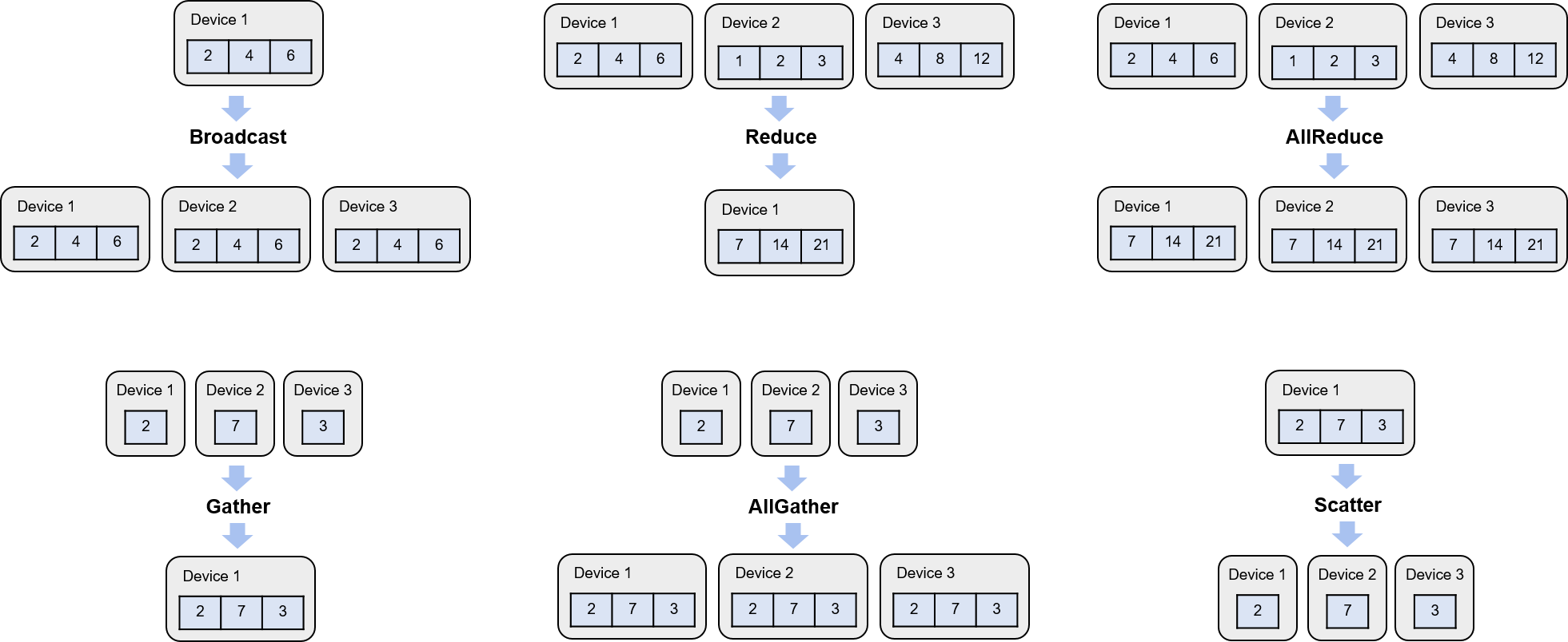
Fig. 8.5.1 Examples of collective communicationoperators
Broadcast: The Broadcast operator is often employed in a distributed machine learning system to transmit model parameters or configuration files from device \(i\) to all other devices. The starting and final states of this operation, initiated by device 1 in a three-device cluster, are depicted in Figure Fig. 8.5.1.
Reduce: In a distributed machine learning system, the Reduce operator plays a pivotal role by consolidating computation results from different devices. It is commonly used to aggregate local gradients from each device to compute the gradient summation. This operator employs functions, represented as \(f\), which often obey the associative and commutative laws. Such functions, including sum, prod, max, and min, are initiated by all devices, with the final aggregate result stored in device \(i\). The initial and final states when device 1 executes the Reduce operator for summation are depicted in Figure Fig. 8.5.1.
AllReduce: The AllReduce operator, a part of collective communication, stores the result of the Reduce function \(f\) in all devices. Figure Fig. 8.5.1 shows the starting and ending states when devices 1, 2, and 3 jointly execute AllReduce to perform a summation.
Gather: The Gather operator can gather data from all devices and store it in device \(i\). Figure Fig. 8.5.1 shows the initial and end states when device 1 invokes the Gather operator to gather data from all devices.
AllGather: The AllGather operator sends the gather result to all devices. Figure Fig. 8.5.1 shows the initial and end states when devices 1, 2, and 3 invoke the AllGather operator.
Scatter: The Scatter operator is the inverse of the Gather operator. Figure Fig. 8.5.1 shows the initial and end states when device 1 invokes the Scatter operator.
It’s important to note that other collective communication operators may also be deployed in distributed machine learning applications. Examples of these are ReduceScatter, Prefix Sum, Barrier, and All-to-All. However, this section will not delve into the specifics of these operators.
8.5.2. Gradient Averaging with AllReduce
The following discusses how to utilize AllReduce operators to implement efficient gradient averaging in large clusters. We can implement a simple method for computing the average gradient, whereby a device in the cluster gathers local gradients from each device and then broadcasts the computed average gradient to all devices. Although this approach is easy to implement, it leads to two problems. 1) Network congestion may occur if multiple devices send data to the gather device simultaneously. 2) It is not feasible to fit gradient averaging computation on a single device due to the computing power constraint.
To solve the preceding problems, the Reduce-Broadcast implementation of the AllReduce operator can be used to optimize the algorithm. In this implementation, all nodes participate in network communication and averaging computation of gradients so that the huge amount of network and computing overheads is evenly shared across all nodes. This implementation can solve the two problems of a single gradient gather node. Assume that there are \(M\) devices, and that each device stores a model replica consisting of \(N\) parameters/gradients. According to the requirements of AllReduce, all parameters need to be partitioned into \(M\) partitions based on the number of devices, with each partition containing \(N/M\) parameters. The initial and end states of the algorithm are provided.
In the AllReduce example shown in Figure Fig. 8.5.1, there are three devices. Each device has a model replica, and each replica has 3 parameters. According to the partitioning method of AllReduce, parameters are partitioned into three partitions (because there are 3 devices), and each partition has 1 (\(N/M\) = 3/3) parameter. In this example, assume that device 1 has parameters 2, 4, and 6; device 2 has parameters 1, 2, and 3; and device 3 has parameters 4, 8, and 12. After an AllReduce operator is used for computation, the gradient summation results 7, 14, and 21 are sent to all devices. The result 7 of partition 1 is the sum of the initial results of partition 1 in the three devices (7 = 1 + 2 + 4). To compute the average gradient, the sum of gradients needs to be divided by the number of devices (e.g., to obtain the final result of partition 1, divide 7 by 3).
The AllReduce operator splits the gradient computation into \(M-1\) Reduce operators and \(M-1\) Broadcast operators (where \(M\) indicates the number of nodes). Reduce operators are used to compute the summation of gradients, and Broadcast operators are used to broadcast the summation of gradients to all nodes.
Figure Fig. 8.5.2 shows the execution process of an AllReduce operator. The AllReduce operator starts with a Reduce operator. In the first Reduce operator, the AllReduce operator performs pairing on all nodes and enables them to jointly complete gradient summation. In the first Reduce operator shown in Figure Fig. 8.5.2, devices 1 and 2 are paired to jointly complete the summation of data in partition 1. Device 2 sends local gradient data 1 to device 1, which adds up the received gradient data 1 and gradient data 2 stored in local partition 1 to obtain the intermediate gradient summation result 3. At the same time, devices 1 and 3 are paired to jointly complete the summation of data in partition 3, and devices 3 and 2 are paired to jointly complete the summation of data in partition 2.
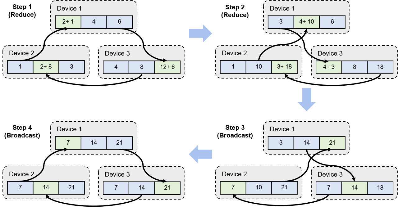
Fig. 8.5.2 Process of the AllReducealgorithm
Such distributed computing of gradients performed by Reduce operators realizes the following performance optimizations:
Network optimization: All devices receive and send data simultaneously by utilizing their ingress and egress bandwidths. Therefore, in the execution process of the AllReduce algorithm, the available bandwidth is \(M * B\), where \(M\) indicates the number of nodes and \(B\) indicates the node bandwidth. This enables the system to implement network bandwidth scalability.
Computing power optimization: Processors of all devices participate in the gradient summation. Therefore, in the execution process of the AllReduce algorithm, the total number of available processors is \(M * P\), where \(M\) indicates the number of nodes and \(P\) indicates the number of processors for a single device. This enables the system to implement computing scalability.
Load balancing: Data partitions are evenly partitioned. Therefore, the communication and computing overheads allocated to each device are the same.
In the Reduce operators other than the first one, the AllReduce algorithm selects other pairing methods for different data partitions. For example, in the second Reduce operator shown in Figure Fig. 8.5.2, the AllReduce algorithm pairs devices 1 and 3 for data summation in partition 1. Devices 1 and 2 are paired for data summation in partition 2, and devices 2 and 3 are paired for data summation in partition 3. In a three-node AllReduce cluster, after two Reduce operators complete execution, the data summation result of each partition is obtained. The data summation result (7) of partition 1 is stored on device 3, the data summation result (14) of partition 2 is stored on device 1, and the data summation result (21) of partition 3 is stored on device 2.
The AllReduce algorithm then enters the broadcast phase. The process in this phase is similar to the execution process of Reduce operators. The core difference is that, after nodes are paired, they do not add up data — instead, they broadcast the computation results of Reduce operators. In the first Broadcast operator shown in Figure Fig. 8.5.2, device 1 directly writes the result (14) of partition 2 to partition 2 of device 3. Device 2 directly writes the result (21) of partition 3 to device 1, and device 3 directly writes the result of partition 1 to device 2. In a three-node AllReduce cluster, the Broadcast operator is repeated twice in order to notify all nodes of the Reduce computation result of each partition.
8.5.3. Model Training with Collective Communication
Typically, a machine learning system flexibly combines different collective communication operators for different clusters to maximize communication efficiency. The following describes two cases: ZeRO and DALL-E.
ZeRO is a neural network optimizer proposed by Microsoft. In practice, ZeRO successfully trained the world’s largest language model in 2020 (with up to 17 billion parameters). In the training process of a neural network like this, parameters of the optimizer, gradients obtained during backward computation, and model parameters all impose significant pressure on the memory space of accelerators. If parameters are represented by 32-bit floating-point numbers, a model with 17 billion parameters requires at least 680 GB of memory, far exceeding the maximum memory capacity (80 GB) of NVIDIA A100 (an accelerator with the largest memory available today). Therefore, we need to explore how to efficiently split a model across different accelerators, and how to efficiently utilize collective communication operators for model training and inference. The following describes three optimization technologies regarding collective communication:
Parameter storage on a single node: The bandwidth of the accelerators inside a node in a modern cluster is much greater than the inter-node bandwidth. Therefore, we need to minimize inter-node communication and ensure that communication mostly happens between accelerators inside nodes. The model slicing process shows that the amount of communication between different slices during the forward and backward computation of the model is far less than the average amount of communication required for gradient averaging of model replicas. As such, ZeRO stores all slices of a single model in the same node, greatly improving the training efficiency.
Forward computation based on the AllGather operator: Assuming that the parameters in a model are linear by layer, we can assign the parameters to different accelerators from front to back based on the sequence of these parameters on the network. In forward computation, the computation of a layer depends only on the parameters of its adjacent layers. Given this, we can apply AllGather computation once on all accelerators that contain model parameters in order to extract the parameters of the next layer for the current layer and to compute the activation value of the current layer. To conserve memory resources, the parameters of layers other than the current one need to be discarded immediately after the AllGather operation is complete.
Gradient averaging based on the ReduceScatter operator: Similarly, during backward computation, only the parameters of the previous layer are needed to compute the activation value and gradient of the current layer. Therefore, AllGather can be used again to complete the gradient computation on each accelerator. At the same time, after gradients are gathered, each accelerator needs only the gradient corresponding to the layer with the same index as the accelerator. In this case, the ReduceScatter operator, instead of AllReduce, can be used to directly store the corresponding gradient to accelerator \(i\).
DALL-E is a text-based image generation model proposed by OpenAI. This model has up to 12 billion parameters. In addition to the AllGather + ReduceScatter technique used by ZeRO during training, the OpenAI team made further optimizations. The following describes two optimization technologies regarding collective communication:
Matrix factorization: The operational speeds of collective communication operators are positively correlated with the message length. In model training, the message length indicates the number of model parameters. DALL-E uses matrix factorization to convert a high-dimensional tensor into a two-dimensional matrix, and then uses collective communication operators for transmission after factorization. In this way, DALL-E significantly reduces the amount of communication.
Custom data types: Another way to reduce the amount of communication is to modify data types. As expected, the 16-bit half-precision floating-point number representation can reduce the amount of communication by nearly half compared with the 32-bit floating-point number representation. However, in practice, low-precision data types cause unstable model convergence and compromise the final training result. OpenAI analyzes the structure of the DALL-E model and classifies the model parameters into three categories based on their sensitivity to the precision of data types. The most precision-sensitive parameters are represented by 32-bit floating-point numbers and synchronized only by the AllReduce operator, whereas the most precision-insensitive parameters are compressed and transmitted using matrix factorization. For the remaining parameters, such as the moments and variance parameters involved in Adam optimization, OpenAI implements two new data types based on the IEEE 754 standard: 1-6-9 and 0-6-10. (The first digit indicates the number of bits required for expressing positive and negative, the second digit indicates the number of bits required for expressing the exponent, and the third digit indicates the number of bits required for expressing a valid number.) In addition to conserving space, this also ensures training convergence.