11.3. Recommendation Pipeline
A recommendation pipeline, designed to suggest items of potential interest to users based on their requests, is an integral part of any recommender system. Specifically, a user seeking recommendations submits a request that includes their user ID and the current context features, such as recently browsed items and browsing duration, to the inference service. The recommendation pipeline uses these user features and those of potential items as input for computation. It then derives a score for each candidate item, selects the highest-scoring items (ranging from dozens to hundreds) to form the recommendation result, and delivers this result back to the user.
Given that a recommender system generally contains billions of potential items, using just a single model to compute the score of each item necessitates a trade-off between model accuracy and speed. In other words, opting for a simpler model may boost speed but potentially result in recommendations that fail to pique the user’s interest due to diminished accuracy. On the other hand, using a more complex model may provide more accurate results but deter users due to longer waiting times.
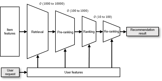
Fig. 11.3.1 Example of a multi-stage recommendationpipeline
To mitigate this, contemporary recommender systems typically deploy multiple recommendation models as part of a pipeline, as illustrated in Figure Fig. 11.3.1. The pipeline begins with the retrieval stage, employing fast, simple models to filter the entire pool of candidate items, identifying thousands to tens of thousands of items that the user may find appealing. Following this, in the ranking stage, slower, more complex models score and order the retrieved items. The top-scoring items (the exact number may vary depending on the specific service scenario), numbering in the dozens or hundreds, are returned as the final recommendation. If the ranking models are too intricate and cannot process all retrieved items within the given time frame, the ranking stage may be further divided into three sub-stages: pre-ranking, ranking, and re-ranking.
11.3.1. Retrieval Stage
The retrieval stage is the initial phase of the recommendation process. The model takes user features as input and performs a rough filter of all candidate items to identify those the user might be interested in. These selected items form the output. The main goal of the retrieval stage is to reduce the pool of candidate items, thereby lightening the computational load on the ranking model in the subsequent stage.
11.3.1.1. Two-Tower Model
To illustrate the retrieval process, let’s consider the two-tower model as an example, as shown in Figure Fig. 11.3.2. The two-tower model contains two multilayer perceptrons (MLPs) which encode user features and item features, referred to as the user tower 1 and item tower, respectively.
Continuous features can be input directly into the MLPs, while discrete features must first be mapped into a dense vector using embedding tables before being fed into the MLPs. The user tower and item tower process these features to generate user vectors and item vectors, respectively, each representing a unique user or item. The two-tower model employs a scoring function to evaluate the similarity between user vectors and item vectors.
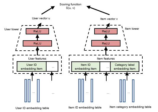
Fig. 11.3.2 Structure of the two-towermodel
11.3.1.2. Training
During training, the model input consists of the user’s feedback data on historical recommendation results, represented by the tuple <user, item, label>. The label denotes whether the user has clicked the item, with 1 and 0 typically representing a click and non-click, respectively. The two-tower model uses positive samples (i.e., samples where the label is 1) for training. To obtain negative samples, an intra-batch sampler that corrects sampling bias performs sampling within the batch. The details of the algorithm, while not the focus here, can be found in the original paper.
The model’s output consists of the click probabilities for different items. During training, a suitable loss function is chosen to ensure that the predicted results for positive samples are as close to 1 as possible, and as close to 0 as possible for negative samples.
11.3.1.3. Inference
Before inference, item vectors for all items are computed and saved using the trained model. Given that item features are relatively stable, this step can reduce computational overhead during inference and speed up the process. User features, which are related to user behavior, are processed when user requests arrive. The two-tower model uses the user tower to compute current user features and generate the user vector. The same scoring function used during training is then used to measure similarity. This enables similarity search based on the user vector across all candidate item vectors. The most similar items are output as the retrieval result.
11.3.1.4. Evaluation Metrics
A common evaluation metric of the retrieval model is the recall metric when \(k\) items are recalled (Recall@k). This metric essentially quantifies the ability of a model to successfully retrieve the top \(k\) items of interest.
The mathematical definition of Recall@k is expressed as follows:
In this equation, the term “True Positive” (TP) refers to the count of items correctly identified by the model as relevant (i.e., with a true label of 1) among the \(k\) items retrieved. On the other hand, “False Negative” (FN) denotes the count of relevant items (again, with a true label of 1) that the model failed to include among the \(k\) retrieved items.
Thus, the Recall@k metric serves as a measure of the model’s ability to correctly identify and retrieve positive samples. Importantly, it is crucial to understand that if the total number of positive samples surpasses \(k\), the maximum possible count of correctly retrieved items is \(k\). This is due to the fact that the model is limited to retrieving only \(k\) items. Consequently, the denominator in the Recall@k equation is defined as the lesser of two quantities: the sum of true positives and false negatives, or \(k\).
11.3.2. Ranking Stage
During the ranking phase, the model appraises the items gathered in the retrieval stage, evaluating each individually in terms of user features and item features. Each item’s score is indicative of the probability that the user might be interested in that item. As a result, the highest-scoring items based on these rankings are then suggested to the user.
If the number of candidate items evaluated by the recommendation model continually increases, or if the recommendation logic and rules become more complex, the entire ranking stage can be efficiently divided into three sub-stages: pre-ranking, ranking, and re-ranking.
11.3.2.1. Pre-ranking
Acting as an intermediary between the retrieval and ranking stages, the pre-ranking stage serves as an additional layer of filtering. This becomes particularly useful when there’s a large influx of candidate items from the retrieval stage, or when multi-channel retrieval methods are used to boost retrieval result diversity. If every retrieved item was directly fed into the ranking model, the subsequent process could become overly lengthy due to the sheer volume of items. Thus, introducing a pre-ranking stage to the recommendation pipeline reduces the number of items proceeding to the ranking stage, enhancing overall system efficiency.
11.3.2.2. Ranking
Ranking, the second stage, is pivotal in the pipeline. In this phase, it’s essential that the model precisely represents the user’s preferences across varying items. When referring to the “ranking model” in subsequent sections, we are specifically addressing the model used during this ranking sub-stage.
11.3.2.3. Re-ranking
In the final re-ranking stage, the preliminary outcomes derived from the ranking stage are further refined according to specific business logic and rules. The goal of this stage is to improve the holistic quality of the recommendation service, shifting the focus from the click-through rate (CTR) of a single item to the broader user experience. For instance, the applied business logic might include efforts to increase the visibility of new items, filter out previously purchased items or watched videos, and create rules to diversify the order and variety of recommended items, thereby decreasing the frequency of similar item recommendations.
11.3.3. Ranking with Deep Learning
The ranking stage in a recommender system has largely benefited from the use of deep learning models. These models are often referred to as the Deep Learning Recommendation Model (DLRM). As depicted in Figure Fig. 11.3.3, a DLRM consists of embedding tables, multi-layer perceptrons (MLPs) that include two layers, and an interaction layer. 2
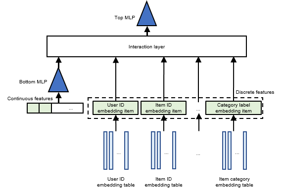
Fig. 11.3.3 Structure of DLRM
Similar to the two-tower model, the DLRM initially uses embedding tables to transform discrete features into corresponding embedding items, which are represented as dense vectors. The model then combines all continuous features into a single vector, which is introduced into the bottom MLP, generating an output vector with the same dimension as the embedding items. Both this output vector and all the embedding items are then forwarded to the interaction layer for further processing.
As illustrated in Figure Fig. 11.3.4, the interaction layer performs dot product operations on all features (encompassing all embedding items and the processed continuous features) to obtain second-order interactions. As the features interacted within the interaction layer are symmetric, the diagonal represents each feature’s self-interaction result. In the non-diagonal section, every distinct pair of features interacts twice (e.g., for features \(p\) and \(q\), two results are acquired: \(<p,q>\) and \(<q,p>\)). Therefore, only the lower triangular part of the result matrix is retained and flattened. This flattened interaction result is merged with the output from the bottom MLP, and the combined result is used as the input for the top MLP. After further processing by the top MLP, the final output score reflects the probability of a user clicking on the item.
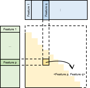
Fig. 11.3.4 Interaction principlediagram
11.3.3.1. Training Process
The DLRM bases its training on <user, item, label> tuples. It takes in user and item features as inputs and interacts with these features to predict the likelihood of a user clicking an item. For positive samples, the model aims to approximate this probability as closely to 1 as possible, while for negative samples, the goal is to get this probability as near to 0 as possible.
The ranking process can be considered a binary classification problem; the (user, item) pair can be classified either as click (label: 1) or no click (label: 0). Therefore, the method used to evaluate a ranking model is analogous to that employed for assessing a binary classification model. However, it’s crucial to consider that recommender system datasets tend to be extremely imbalanced, meaning the proportion of positive samples is drastically different from that of negative samples. To minimize the influence of this data imbalance on metrics, we use the Area Under the Curve (AUC) and F1 score to evaluate ranking models.
The AUC is the area under the Receiver Operating Characteristic (ROC)
curve, a graph used to define classification thresholds, plotted with
the True Positive Rate (TPR) against the False Positive Rate (FPR) —
with the TPR on the y-axis and the FPR on the x-axis. An appropriate
classification threshold can be determined by calculating the AUC and
the ROC curves. If the predicted probability exceeds the classification
threshold, the prediction result is 1 (click); otherwise, it is 0 (no
click). From the prediction result, recall and precision can be
computed, which in turn allows for the calculation of the F1 score using
the formula f1.
:eqlabel:equ:f1
11.3.3.2. Inference Process
During the inference stage, the features of the retrieved items, along with their corresponding user features, are merged and inputted into the DLRM. The model then predicts scores, and the items with the highest probabilities are selected for output.